Accuracy and Checking in FEA, Part 1
The final accuracy of the results reported in a finite element analysis model depends on many factors. Let's take a look at how errors can occur -- and how to avoid them.


January 1, 2014
By Tony Abbey
Editor’s Note: Tony Abbey teaches live NAFEMS FEA classes in the US, Europe and Asia. He also teaches NAFEMS e-learning classes globally. Contact [email protected] for details.
In the finite element analysis (FEA) process, checking is done at every stage. Before the analysis even starts, we need to get all our material data, dimensions, masses, loading definitions and other data clearly organized.
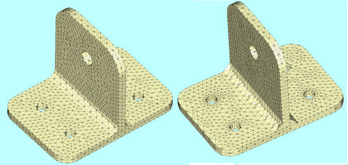 Fig. 1: Good- and poor-quality meshes. |
Obtaining accurate and validated data can take a surprisingly long time. Start the project report early, and include this information as it becomes available. I have written reports at the last minute, and found the wrong material properties used in the model. There is no choice, then, but to re-run the analysis—with a strong possibility that all results will have changed.
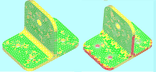 Fig. 2: Element aspect ratio check plots. |
In the pre-processing stage, we mesh the model. We apply loads and boundary conditions, material properties, etc. We can do many checks here. The first check during meshing is to assess element quality; distorted element shapes are our biggest enemy.
What do we mean by “quality,” and why is this important? In the calculation of the overall structural stiffness, each element is evaluated numerically. The accuracy of the element stiffness—and hence, the accuracy of the whole model—depends on how well this element evaluation is carried out.
Good and poor quality meshes are shown in Fig. 1. We can see by eye that one mesh is inferior, but applying more formal checking is better practice. Fig. 2 shows a typical checking element criterion plot (using aspect ratio), highlighting the poor mesh.
A large number of element checking formats are available. One of the best catch-all methods is element aspect ratio. If this is set to a high number, such as 10, it will trap all of the rogue elements that are often created in a mesh. This includes sliver-type element shapes, or collapsed elements, where the mesher has become confused by poor geometry or tolerance errors. Fig. 3 shows a typical aspect ratio definition of longest over shortest length. A word of caution here: The pre-processor definition may be different from the solver definition, which is the important version.
General Performance
Once we have removed obviously bad elements, we can check the general performance of the mesher. Many meshers are able to show mesh quality interactively. This is extremely useful, as it helps guide us toward improvements in the mesh. If we are meshing 3D elements, it is important that we are checking the shape of elements in the interior of the geometry. Fig. 4 shows a typical case where the mesh looks fine on the outside, but is very poor inside. Splitting the mesh apart visually is the only way to see this.
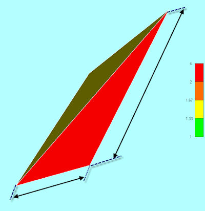 Fig. 3: Typical aspect ratio definition of a 3D tetrahedral element. |
Some meshers enhance our ability to check inside the mesh by providing a slider bar to control which elements we see. Setting an aspect ratio value will only show elements that are above that threshold. Fig. 5 shows a typical example. Grouping or color-coding these elements are another powerful tool to help us identify and improve the mesh.
Jacobian Calculations
Perhaps the most powerful element checking format is the Jacobian. Unfortunately, it is also the most difficult to interpret and expensive to calculate. Each element forms a Jacobian matrix during the evaluation of its stiffness matrix. This is, therefore, a direct representation of how numerically accurate the element is.
All geometric factors play a part in this. With a large model, the cost of emulating the Jacobian calculations in the preprocessor can become prohibitive.
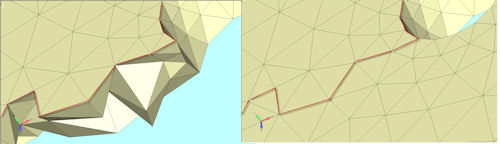 Fig. 4: Smooth external mesh hides poor internal mesh. Split line is shown. |
It is important to understand that this is an emulation, not the actual solver calculation. You may find controls such as “approximate” or “accurate” calculation options. The evaluation may just use faces of 3D elements. It is important to experiment with controlled mesh distortions to evaluate for yourself just how effective the “approximate” calculations are compared to the resultant analytical values.
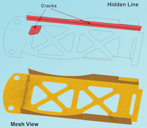 Fig. 5: Highest criteria set on the left, lowest on the right. |
The fundamental question is: What is a good Jacobian value? Unfortunately, it is not possible to define that in a general sense. The value is definition-, element type-, dimensional- and solver-specific. The best way to approach this, then, is to experiment and calibrate mesh distortions yourself, to build a good baseline. Fig. 6 shows a typical study.
Model Cracks
Cracks in a mesh occur where adjacent elements are not properly connected. Reasons include differences between tolerances in the CAD model and FEA models, and mismatched element mesh densities between adjacent surfaces or volumes. Most meshers will refuse to collapse an element, so awkward junctions of element shapes may resist attempts to join up nodes that are very close to each other.
 Fig. 6: A family of progressively distorted tetrahedral elements, with Jacobian checks. |
It is important to preview cracks as the meshing occurs. Most meshes will allow snapping between free edge or free face view and normal view. Fig. 7 shows a typical mesh with a variety of cracks that need to be fixed.
Element Normals
Each 2D element (or face in a 3D element) has a normal or perpendicular direction. The element normal is used to define several important characteristics in the analysis. The most obvious is the direction to apply a pressure load in a 2D element.
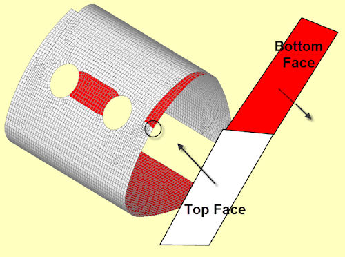 Fig. 7: Full mesh view and free edge hidden line view, showing cracks. |
A typical convention uses the pressure direction running into the element, against the element normal. This is shown in Fig. 8. The resultant normal for each geometry face is somewhat arbitrary when meshing the typical complex 2D geometry found in a component. If we want to apply consistent pressure loading, it is important to check the sense of the normal—and hence, the pressure load—and if necessary, reverse the sense. We can plot the element normal as a vector, but for a complex model, this ends up looking somewhat like a porcupine!
A better way is to paint the back faces of elements with a distinct color. This is shown in Fig. 8, where pressure loading is clearly shown to be in error and the correction can be made.
The other important use of an element normal in a 2D element is to define the top and bottom surfaces. A bending moment applied to the element will result in tension and compression surface stresses. Consistent element normals are required to get the correct post-processing stress distributions.
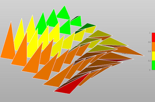 Fig. 8: Element normal with back faces painted red. Notice the errors in pressure load directions. |
Finally, element normals are also used to define offsets, and stacking orientation in composite layups. Mixing up normals will cause random errors in all of these.
Load Balance
It is important to make sure that we have the loading defined correctly. Some loading forms are straightforward, with just a few isolated loads. However, the loading can get quite complex with distributed pressure loading, body inertia loading, etc. In all cases, we want to check the magnitude and resultant line of action of the loading against our specification. We can check visually, using the preprocessor graphics to make sure the distribution of the loading is correct.
Many preprocessors provide a load balance check tool to make sure that we have calibrated the load properly. For example, inaccuracies between geometric area or volume and subsequent mesh area and volume will cause loading errors. We can adjust the loading to match the specification. The definitive check on load balance will occur after the solution, and we will look at that later.
Boundary Conditions
Setting up the correct boundary conditions is also vital for successful analysis. Again, these can be very simple, or complex with local coordinate systems and specific degrees of freedom (DOF) components defined. Throughout 2014 in DE, we will look at various advanced checks using supplementary analyses, production analysis and post-processing.
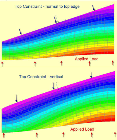 Fig. 9: Constraint is applied in the wrong coordinate system in the lower model. |
In the preprocessor, we can focus on the graphical representation of the constraints. It is a good idea to thoroughly review the constraints at this stage to make sure that nothing has been missed or applied in error. When using automated setup options such as symmetry, I strongly recommend double-checking that you understand and agree with how these options have been setup. Similarly, local coordinate systems are very powerful to describe realistic constraint systems, but they are also very error-prone, as shown in Fig. 9.
Physical, Material and Mass Properties
Checking physical properties, such as shell element thickness and beam cross-sections and material operatives, is largely a matter of housekeeping. But again, we usually have a full set of graphical and tabular options in the preprocessor to help us here. Color-coded mesh plots of property and material distribution are an extremely useful checking option—and also good practice to include in the report.
Beam and shell element idealization features, such as cross-section visualization, orientation vectors and offsets can be checked visually in the preprocessor. This is extremely powerful; spare a thought for engineers of 20 years ago who would be staring at a screen full of lines, trying to check these aspects. I always worried about “Friday afternoon models,” where human nature meant that the error level was probably quite high!
If we are using mass in an analysis, for static inertia loading or dynamic analysis, it is vital that we check the mass distribution. Again, most preprocessors have great tools to help us check this out before we commit to an analysis. Most components will have mass properties stated in the specification, and we can check against these.
It is important to include the mass moments of inertia as well as the mass. If we are using lumped mass idealizations for components, this becomes very important. A common error is to just include the translational mass.
The physical analogy is a large block of steel on ice, which resists a push at its center gravity. However, if we push on an edge, it will spin rapidly, as it has no rotational inertia resistance.
In FEA, there is a lot of checking to do! However, if a consistent and rigorous approach is taken, it will improve the likelihood of creating accurate models—and will also give checkers and reviewers a great deal of confidence.
Tony Abbey is a consultant analyst with his own company, FETraining. He also works as training manager for NAFEMS, responsible for developing and implementing training classes, including a wide range of e-learning classes. Send e-mail about this article to [email protected].
Subscribe to our FREE magazine, FREE email newsletters or both!
About the Author
Tony Abbey is a consultant analyst with his own company, FETraining. He also works as training manager for NAFEMS, responsible for developing and implementing training classes, including e-learning classes. Send e-mail about this article to [email protected].
Follow DE

