An Optimization Overview
Optimization technology has advanced rapidly over the last decade, and engineers face a bewildering variety of tools and methods.


December 1, 2012
By Tony Abbey
While it is tempting to view optimization as a black box—press the button and the “Answer to Life, the Universe and Everything” emerges—sadly, that doesn’t happen often. To understand optimization, we must first ask ourselves some basic questions about our goals, our designs and our constraints.
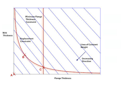 |
| Figure 1: Design space. |
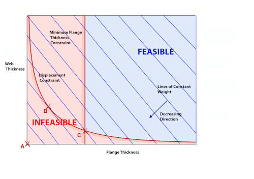 |
| Figure 2: Design space showing feasible and infeasible regions. |
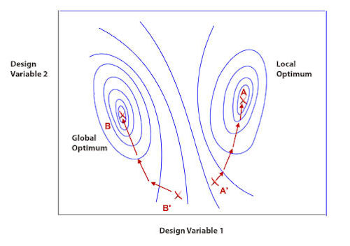 |
| Figure 3: Global and local optima. |
What are we trying to achieve with an optimization?
This is defined by the objective function, and is traditionally weight minimization. It can be many other things, however, such as maximizing strength. Innovative optimization solutions can be found by thinking about the objective function “out of the box.”
Until recently, methods used one unique objective. Allowing multiple objectives is now common—for example, we can evaluate the effect of minimizing weight and at the same time maximizing strength. We don’t often get one unique solution; instead, a set of trade-offs is found, all of which are “best in class.” The trade-offs are shown in a way that can be investigated to help the user make a decision. The user chooses a compromise between weight and strength margin.
How do we define what we want optimized?
The set of parameters that define the optimization task are called design variables. We will see examples across a wide range of optimization types. But for now, imagine a 2D shell model, such as a storage tank, plating in a girder bridge, etc. Each different plate thickness will be defined by a design variable. For the tank, it may be a single design variable; for the bridge, it may be the separate flange, and shear web thicknesses define two design variables. We may allow more thickness variation and increase the design variable count.
What restrictions do we want to put on the structure?
Restrictions are defined as optimization constraints (not to be confused with structural constraints). There are two types: response constraints, preventing the structure from violating stress limits, displacement values, frequencies, etc., and gage constraints, limiting the model’s physical parameters such as wall thickness and beam cross-sectional area.
Constraints can be upper- or lower-bound, a wall thickness defined between upper and lower design limits. Displacement may be limited to a maximum and minimum value. A small tolerance is sneaked in here—it is expensive to trap exact values.
Optimizers hate equality constraints, such as displacement or stress forced to match specific values. It provides a big numerical challenge, so another small tolerance is sneaked in.
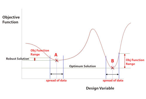 |
| Figure 4: Robust design vs. optimum design. |
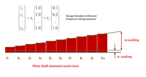 |
| Figure 5: Design variable linking. |
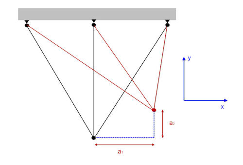 |
| Figure 6: Three-bar truss showing shape variables. |
After all these questions, we may have a bridge structural model, optimized to minimize the weight. The bridge maximum stresses must not exceed a limiting level, and the center deflection must be below an upper limit. The two design variables are flange and web thickness, defined by the property associated with the relevant elements.
Design Space
Design space is shown schematically in Fig. 1 for the bridge. The design variables form the axes, and lines of constant weight are plotted. Without constraints, we have a silly optimum zero weight at A. Adding a displacement constraint gives us a practical design, and the optimum is B. A minimum constraint on flange thickness moves us to a heavier solution, C. Designs that are outside the constraints are feasible; those violating one or more constraints are infeasible, as shown in Fig. 2.
The bridge objective function is linear with a constant gradient. That makes searching for the optimum easy by following the gradient until finding a constraint and sliding down it until we can’t go any further. That forms the basis of an important class of methods, gradient methods. These are very powerful when used in internal optimization engines embedded within an finite element (FE) solver. The gradients can be solved analytically rather than numerically, saving computational resource and optimization steps. Each optimization step means a reanalysis. Typical gradient methods may need 10 to 20 steps.
A big drawback of gradient methods is that we cannot be sure of a global optimum. Fig. 3 shows an optimum at A, given a start at A’. If we start at B’, then we find B, which is the best or global optimum.
Gradient methods can have multiple starting points, but there is still no guarantee of a global optimum—and the cost increases.
A powerful range of methods, taking very different approaches, has been introduced into optimization and are better suited to finding a global optimum. These methods are typically found in external optimization tools, which drive FEA and potentially other parallel multi-disciplinary simulations. The list includes:
- Genetic algorithms use survival of the fittest, reproduction and mutation simulations to evolve an optimum design. The design variables are codified, usually via binary numbers, in a gene-like representation. Radical designs can evolve from this method. Limited sets of gage sizes are well handled—often a problem for gradient methods.
- Neural networks use a simulation of the brain’s neural paths. The system is trained on a set of analyses and learns what constitutes a “good” solution. Again, radical designs can be produced; gage sets are ideal and even invalid analyses will be recognized.
- Design of experiments (DOE) uses an initial scattershot approach across design space. This can intelligently evolve into a set of solution points that characterize design space, and this “curve fit” is used to find a global optimum.
The downside of these methods is that huge numbers of FEA solutions are needed, often in the thousands. However, with increasing computing power, many structural models are now viable. They can provide radical solutions, but the “thought process” is not easily traceable, unlike gradient methods.
Keeping Optimum’ in Perspective
Much early work focused on mathematical search methods using well-defined benchmark problems, and to some extent concentrated on getting the best “optimum” solution to high significant figures. To put that in perspective, “good” FEA may give us stress results to around 5% accuracy!
Modern approaches now include searching to improve the robustness of an optimum solution, as well as the raw “best value.” Fig. 4 shows the basis of the method. Design A is the “best,” as it minimizes the objective. However, it is unpredictable with small variations in input parameters—remember, we struggle to simulate the real world, and may also in fact end up violating a constraint such as stress or displacement.
We also need to keep an intuitive feel for the robustness of an optimization analysis. One trap is to miss some of the loading cases applied. Unfortunately, the resultant “optimized” structure is very likely to fail when the full load set is applied, as it has been carefully designed to ignore it. Similarly, any poor assumptions or idealizations in the baseline FEA model may well be exaggerated. It is worth spending additional time debugging this model before going onto an optimization study.
Topology optimization is probably the most radical, “free spirit” approach, and is often used in conceptual design. At the other end of the scale, sizing optimization is tuning a fixed layout, and may be used as a final pass in an optimization process.
How FEA Carries out Optimization Analysis
The various approaches to optimization found in FEA are basically defined by the way the design variables are used. The earliest method used the simplest parameters available to control the FEA model’s physical properties, including:
- shell thickness;
- rod or beam area;
- beam second moments of area; and
- composite ply angles and thicknesses.
Sizing Optimization
The design variables are limited to the idealization parameters of bars, beams, shells, etc.—1D and 2D elements. This type of optimization is called sizing optimization, sizing the property parameters. This method is widely used in aerospace, maritime and anywhere the 1D and 2D idealization dominates.
The linking of design variables to property parameters can be a simple direct relationship, or a more complex combination of many parameters. Fig. 5 shows linking shell thicknesses for a tapering skin.
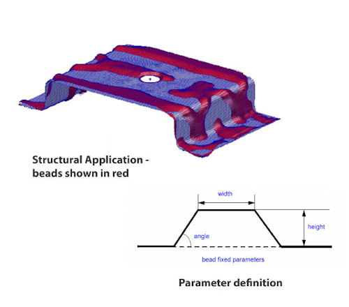 |
| Figure 7: Bead definition and application. |
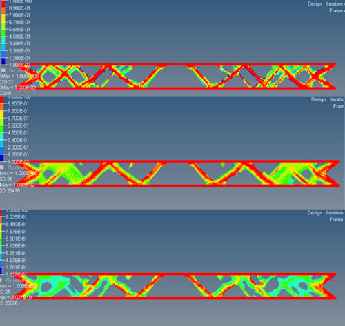 |
| Figure 8: Topology variations in a beam structure, plotted as relative material stiffness. |
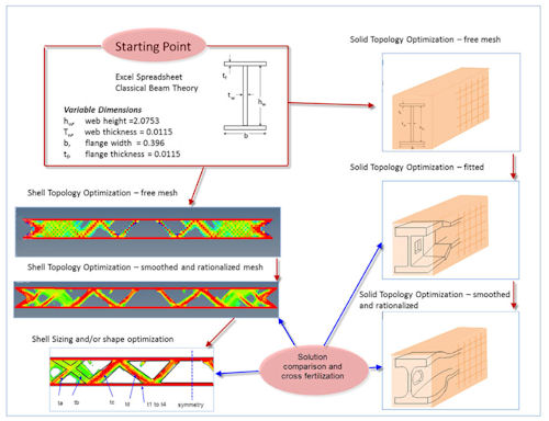 |
| Figure 9: Comprehensive workflow to study project optimization. |
Shape Optimization
Shape optimization controls the nodal positions of 1D, 2D and 3D structural meshes. Until recently, the FE models kept the same mesh, but the mesh could be distorted. Fig.6 shows a simple 1D example. The two design variables a1 and a2 are the node position in x and y.
If we have a more general mesh with many nodes, however, the definition of design variables becomes at first tedious—and then rapidly impossible. Simplification schemes such as giving linear control over edges through nodal position linking can be used.
An alternative approach introduces an “auxiliary model.” The parent mesh is distorted in arbitrary, but “natural” ways by applying loading or using mode shapes. The load case on the auxiliary model has no meaning other than to give “pretty shapes.” These shapes are then combined and scaled in the optimization to give the final structural mesh shape. Some dexterity is required to set up sensible auxiliary analyses.
Thankfully, recent advances in shape optimization allow morphed variants of the mesh, either directly from the original mesh or via parent geometry morphing.
Another innovation uses a restrictive movement of nodes in shell-type structures to give a beading or swaging effect. Fig. 7 shows nodes allowed to move a fixed amount in a fixed direction. The result is a very useable tool to represent thin panel stiffening, with simple user input defining the design variables.
Shape optimization usability is greatly increased by a new approach. Instead of minimizing weight as the objective function, a weight reduction target is set at, say, 40%, and the objective is to achieve a homogeneous distribution of stress or energy. This can be coupled with automatic perturbation of edge nodes (2D) or surface nodes (3D) and automatic remeshing.
The remeshing operation blurs the original definition of shape optimization. It also has the benefit of avoiding a drawback of shape optimization: excessive element distortion.
Topology Optimization
An alternative to directly controlling size or shape parameters via design variables is to provide a fixed 2D or 3D design space filled with elements. The elements can be “removed” to evolve the structural configuration.
A traditional FE model requires a full mesh of nodes and elements so that the stiffness matrix remains a constant size. Element removal is “faked” by reducing effectiveness. Typically, Young’s Modulus and density is reduced, so that a resultant structural configuration of, say, steel is surrounded by mathematical chewing gum. Typical results are shown in Fig. 8, with various parameters controlling the width of members and the sharpness of the material transition.
Topology optimization has also been transformed by replacing traditional weight minimization with maximizing stress or strain energy “smoothness.”
The final technology improvement has been to take the “LEGO Brick” mesh results (formed by elements removed in a mesh) and fit usable geometry through the surface nodes. Likely improvements over the next few years include automatic parameterization to increase the relevance to real design and manufacturing geometry.
The Science and Art of Optimization
Engineers are faced with a wide range of optimization methods, including shape, sizing and topology. The underlying technology can vary from gradient methods to neural networks. Some methods have very synergistic technologies—shape and gradient or topology and GA. However, it is up to the user to look carefully at the guidance and recommendations in supporting documentation. The full list of technologies can run to 20 or 30 different algorithms. Some external optimizers have strong automatic selection strategies to link the right technology with a method.
The decisions taken in setting up an optimization problem will strongly influence the optimum found; there is no single right answer. The best we can hope for is to use a combination of engineering judgment, good FE modeling and innovative use of optimization software to come up with a design solution that is often a best compromise. The software by itself cannot achieve that. Multi-objective methods can go some way to assisting us down the path, but common sense is still required to avoid making the problem overly complex.
Fig. 9 shows a schematic that moves progressively through logical stages of optimization of a beam, comparing a 2D shell idealization and a full 3D solid idealization.
We are moving from the conceptual design phase, using classical calculations to get into the right ballpark and then opening the design up to more radical solutions with topology optimization, before finally enforcing more discipline on the design via sizing optimization. The last stage provides a manufacturable design and formal structural sign-off.
Alternatively, it can be argued that the use of the spreadsheet and 2D topology of a defined configuration is too restrictive, and more radical designs are sought. Then a 3D topology optimization with GA technology may be the best approach.
The optimum, like beauty, is in the eye of the beholder.
Tony Abbey is a consultant analyst with his own company, FETraining. He also works as training manager for NAFEMS, responsible for developing and implementing training classes, including a wide range of e-learning classes. Send e-mail about this article to [email protected].
Subscribe to our FREE magazine, FREE email newsletters or both!
About the Author
Tony Abbey is a consultant analyst with his own company, FETraining. He also works as training manager for NAFEMS, responsible for developing and implementing training classes, including e-learning classes. Send e-mail about this article to [email protected].
Follow DE

