Conduct Fatigue Analysis using FEA
Calculating structure fatigue and stresses through finite element analysis can help predict weak spots and other potential problems -- before manufacture.


Latest News
June 1, 2013
Editor’s Note: Tony Abbey teaches the NAFEMS FEA live FEA classes in the United States, Europe and Asia throughout the year, and teaches e-learning classes globally. Contact [email protected] for details.
Fatigue is often cited as the most common form of failure in structures. It occurs at relatively low stresses, below the critical static value. But the stresses are cycling, typically between tension and compression. Early research work was motivated by railway axle failures some 170 years ago—and is still being undertaken to bring a fuller understanding of fatigue.
Cyclic loading applied on a structure will result in cyclic local stresses. A railway axle sees compressive loads in the top and tensile in the bottom of the shaft. Rotating 180° reverses the local stresses. A further 180° gives the original local stress state.
The cyclic stress history becomes important when it occurs at a potential crack initiation site. This can be any microscopic level defect or void inherent in the material or introduced by machining or other environmental effects. Damage is accumulated during the loading history of the component. If the damage grows beyond a critical point, the crack will initiate.
Fatigue analysis does not introduce a crack into the finite element model. Instead, it assesses the stress state together with loading and environmental factors for potential crack initiation. A fatigue “failure” is an indication that a crack will start. No calculation is made to explore subsequent crack growth.
A finite element analysis (FEA) is carried out to find local regions of high stress under operating conditions. The maximum and minimum stresses under cyclic loading are considered.
Fig. 1 shows a cyclic stress variation. The stress range spans the most positive and negative stresses. Stress amplitude oscillates about a mean stress level. A stress cycle, then, occurs between adjacent peaks.
The number of stress cycles, together with the stress amplitude, dictates the fatigue life of the structure. High-frequency loading is seen in a rotating machine tool. Wave loading on an offshore oil platform is low frequency. Fatigue life could be measured in terms of hours or years, respectively—with both having a similar cycle count at failure.
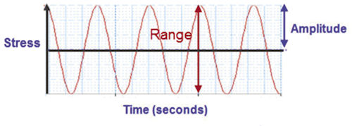 Fig. 1: Typical local stress history. |
Early test data showed a distinct relationship among the stress amplitude (S), the cycle count (N) and the expected fatigue life. This led to the early adoption of the SN curve to predict fatigue (see Fig. 2).
For a stress amplitude (Si) , the number of cycles to failure (Ni) can be calculated. There is a cutoff in the slope at 10^6 or 10^7 cycles, described as the endurance limit. This indicates very low stress amplitudes could achieve an infinite fatigue life. Steels exhibit this behavior. In practice, loading, geometrical and environmental modifiers discussed later may prevent this.
Environmental and Loading Considerations
There are quite a few caveats with the SN curve, however. There is a wide scatter in test results, and the curve is drawn so that 50% of test results lie equally above and below. For more conservative life estimates, a lower percentage line is used.
The test results are for a specific material, condition, environment and loading type. A “raw” SN curve is a baseline on which to apply further factors to obtain a realistic life assessment.
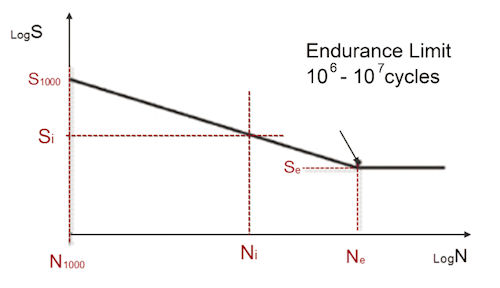 Fig. 2: Stress amplitude vs. fatigue life in cycles. |
Test specimens are often defined as smooth polished. This standard of finish is unlikely in any manufacturing process, so degradation factors are applied to the SN curve. Cast or forged components will have more degradation than high-quality machined parts.
Other factors have to be assessed and applied. This is probably one of the biggest uncertainties in fatigue calculation: It is easy to enter inappropriate data into a friendly graphical user interface (GUI) and overestimate the fatigue life. My recommendation is to seek training or advice, and obtain a good textbook such as “Fundamentals of Metal Fatigue Analysis” (Bannantine, et al. Prentice Hall 1990. ISBN 0-013-340191-X).
Many manufacturers and certification organizations go further than material specimen tests, which are difficult to match to actual conditions. Component tests allow more specific understanding of factors affecting fatigue life. A full-scale fatigue test may be used on the complete assembly. Finite element analysis plays an important role in helping to correlate stresses (and hence, fatigue) at each level.
High-cycle vs. Low-cycle Fatigue
If local stresses are low enough and within the elastic region, a component may have a long fatigue life measured in hundreds of thousands of cycles. This was the scenario in the early fatigue work with railway axles, pressure boilers and the like.
This is known as high cycle fatigue. The classic SN curve as described earlier is the main tool. One caution here: Although the SN curve shows a stress at 1,000 cycles, this is simply a lower datum point on the curve and should never be used. If a stress level is indicating a fatigue life below about 50,000 cycles, then the SN curve is not be appropriate and we should investigate using the following alternative method.
In some cases, the loading is more severe and local stresses, at a crack initiation site, do go plastic for at least part of the loading cycle. At this level of loading, the number of cycles to failure is much lower. It could be of the order 50,000 cycles, or even as low as 50 cycles.
This is referred to as low cycle fatigue. It is more recent technology only possible when plastic influences were better understood. Now stress in a load cycle is characterized by both its elastic and plastic response. This produces a nonlinear stress-strain hysteresis loop (see Fig. 3). The amount of plasticity is judged by the “fatness” of the hysteresis loop. A purely elastic cycle is simply a “skinny” linear stress strain curve.
A strain-based approach is used to characterize the load cycle response. Inside a component at the local high stress region, the local material sees a displacement or strain controlled loading from surrounding material. The elastic and plastic strain components can be calculated to give the total strain range across the loading cycle. A maximum and minimum strain replaces maximum and minimum stress.
The EN fatigue life curve is used, shown in Fig. 3. It is similar to the SN curve, but uses strain amplitude. The intercept of the strain amplitude with the EN curve establishes the number of fatigue cycles to failure. Confusingly, the theory and curves are developed in terms of load reversal, equating to half a load cycle, and strain range, which is twice the strain amplitude.
Low cycle fatigue (EN) calculations can predict fatigue lives as low as a few hundred cycles. Using this approach with low stress levels is fine, as only the elastic portion of the elastic/plastic analysis is used and is equivalent to an SN solution.
Mean Stress Effects
For the SN approach, the level of mean stress within a stress cycle is important. If both maximum and minimum stresses are tensile, every part of the loading cycle has a tendency to open and develop a crack. Conversely, if both are compressive, the crack can’t open. In other words: Compressive stresses are beneficial, and a compressive mean stress will extend the fatigue life. A tensile mean stress will reduce the fatigue life.
Mean stress effects are incorporated via an equivalent amplitude stress with zero mean. The basic SN curve can then be used having corrected for mean stress.
Correction methods are also used for the low cycle fatigue calculation using the EN curve; however, these tend not to be so important, as the influence of mean stress is reduced in the presence of plasticity.
Notch Effects
Peak stress levels can be concentrated at very local features, such as a notch or hole. High cycle fatigue can be too conservative using these stresses. The local fatigue mechanism is influenced by factors ignored at the macro level, including notch size, stress level, stress gradient, etc. The stress concentration factor (Kt) is the ratio of elastic peak local stress to average or nominal stress.
Instead of using this, though, a term called the notch factor (Kf) is used. It tends to blunt the elastic stress result and give a longer life. Calculating Kf is complicated, and relies heavily on empirical methods with extra data on notch size, stress gradient and other factors required for estimation.
Low cycle fatigue with more extensive local plasticity tends to blunt the effect of a notch even further. A typical correction methodology uses the Neuber relationship to establish an energy balance between the nonlinear stress strain curve of the material and the local plasticity in the notch.
Unscrambling Load History
Fig. 1 shows a constant amplitude loading. The amplitude and the mean stress level may in fact vary under loading. This may occur in natural blocks of loading, or it may be a random series of events.
For block loading, each block is dealt with separately. The mean stress correction is made and the number of cycles (N) that can be endured at the stress level (S) is found. The ratio of actual cycles seen in this block, n, compared to the total that can be endured, is n/N. This fraction is called the damage ratio. If n/N equals 0.5, then half the fatigue life is used up in that single block.
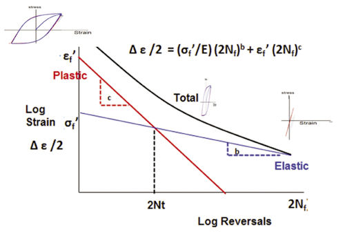 Fig. 3: Low cycle fatigue EN curve showing plastic and elastic contributions. |
The damage ratio from each of the blocks is summed. If total damage is less than 1.0, there is adequate fatigue life. This accumulation process is called Miner’s Law.
Miner’s Law ignores sequencing effects, so a single large load cycle can occur at the beginning or the end of the loading history. In practice, early large levels of load often bring beneficial compressive residual stresses, increasing the fatigue life.
With a more random loading history, a process is required to synthesize equivalent pairs of peaks. One method is rainflow counting. We imagine the load history turned on its side and water dripping down the positive and negative faces. The peak that juts out more will capture a rain drop. That peak is tagged and removed from the load history. A second drip identifies the next highest peak, which is tagged and removed. This process continues until all peaks are removed and is done on both faces. Corresponding peaks from each face are paired to give equivalent cycles.
A similar process is used for low cycle fatigue, but is more complicated because equivalent stabilized hysteresis loops are synthesized.
Going Further
This is a just a brief overview of some of the essential points of fatigue analysis using FEA. Fatigue analysis gets more complicated if the loading history is not a simple linear scaling of one applied load. This leads us onto multi-axial fatigue analysis, which is very much at the cutting edge of technology. Other specializations not described here include fatigue of seam welds, spot welds and bolted joints. Special-purpose, FEA-based tools have been developed to deal with these.
Finally, to investigate a specific crack and evaluate how it will propagate further or stabilize we turn to a complementary analysis methodology: fracture mechanics.
Tony Abbey is a consultant analyst with his own company, FETraining. He also works as training manager for NAFEMS, responsible for developing and implementing training classes, including a wide range of e-learning classes. Send e-mail about this article to [email protected].
More Information
Subscribe to our FREE magazine, FREE email newsletters or both!
Latest News
About the Author
Tony Abbey is a consultant analyst with his own company, FETraining. He also works as training manager for NAFEMS, responsible for developing and implementing training classes, including e-learning classes. Send e-mail about this article to [email protected].
Follow DE

