Fig. 1A and 1B: Loading in either with (1) or transverse to (2), fiber direction.


November 1, 2014
 Fig. 1A and 1B: Loading in either with (1) or transverse to (2), fiber direction.
Editor’s Note: Tony Abbey teaches live NAFEMS FEA classes in the US, Europe and Asia. He also teaches NAFEMS e-learning classes globally. Contact [email protected] for details. Read part 1 of this article here.
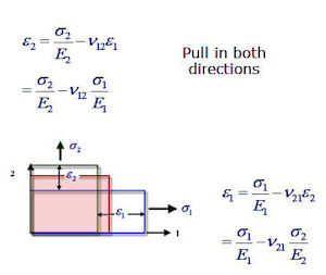 Fig. 2: Loading in both directions at the same time.
The calculation of the stiffness of a laminate or layup is an important step in evaluating a composite finite element analysis (FEA) element. Unlike an isotropic shell element, the stiffness depends on the number and stacking sequence of the individual plies. Each ply can be a varying thickness, angle and material property. The laminate stiffness is also important as a predictor of the response of the composite. Let’s look at how the laminate stiffness is calculated.
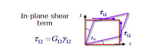 Fig. 3: In-plane shear term.
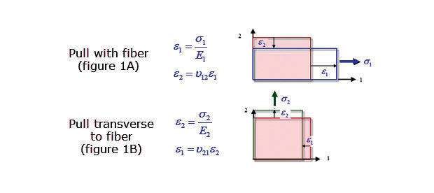
The fundamental building block in a laminate is the ply. For a thin shell calculation, we assume a 2D orthotropic material can represent the ply. The important directions are with-fiber (direction 1) and transverse to fiber (direction 2). Consider a single ply loaded in the with-fiber direction (1) and free to contract in the transverse direction (2) so that transverse stress is zero, but there is a strain because of Poisson’s effect. This is shown in Fig. 1A.
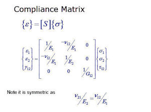 Fig. 4: Compliance matrix definition.
Now consider the ply loaded in the transverse direction (2) and free to contract so that the with-fiber stress (1) is zero, but again there is a strain due to Poisson’s effect. This is shown in Fig. 1B. The equations show that two separate Young’s moduli (E1 and E2) and two Poisson’s ratios are used in the coupling.
Now consider both stresses applied simultaneously. The stresses and strains are shown in Fig. 2. The strain in each direction is coupled between with (1) and transverse (2) terms.
The stress-strain relationship in shear is shown in Fig. 3.
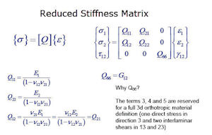 Fig. 5: Ply reduced-stiffness matrix.
If all the stress-strain relationships are combined, the compliance matrix is produced as shown in Fig. 4. Note the relationship between Poisson’s ratios and Young’s moduli. The compliance matrix relates strains to stresses.
To develop a stress-strain relationship, we need to invert this to form a “reduced” stiffness matrix. This is shown in Fig. 5.
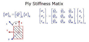 Fig. 6: Ply stiffness matrix.
The act of transforming the ply to an off-axis angle causes a coupling between the shear and direct stress terms, and creates a full ply stiffness matrix. This is shown in Fig. 6, where ply k has been rotated theta degrees. I won’t show the transformation terms, but they are just functions of angle theta.
What is the Matrix?
So, how do we get a laminate stiffness matrix? The final step is to take each 3x3 ply stiffness matrix, factor up by its thickness, and then add all the stiffness terms up. This provides a 3x3 in–plane stiffness matrix that relates applied load (in force/length) to resultant strains. This is called the A matrix. The influence of the A matrix can be seen by considering laminates that are balanced and unbalanced.
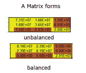 Fig. 7: Balanced and unbalanced in-plane laminate stiffness A matrix.
A balanced laminate has “balanced” ply angle contributions. For example a [5/-5/30/-30/-60/60] laminate has a complete set of +angle/-angle pairs. Note that 0/90 is also a balanced pair. The A matrix is shown in Fig. 7 (lower) and has no coupling between direct and shear stresses as shown by the highlighted zero terms. Even if [5/-5/30/-30/-60/60/60] is used, but the thickness of the single -60 ply is doubled, the laminate is still balanced. Fig. 7 (upper) shows an unbalanced A matrix resulting from [5/-5/30/-35/-60/60].
The physical implication of the A matrix is important; coupling between direct and shear terms means that any direct pull will also result in a shearing action. Any shear will result in a direct stress term. This can cause unwanted stresses in a loaded component—or warped components if thermal curing is used.
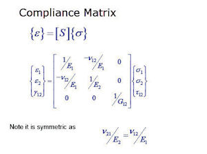 Fig. 8: High and low stiffness bending laminate stiffness terms in D matrix.
The A matrix is also important for calculating equivalent in-plane stiffnesses for hand calculation for rough design estimates, or checking results.
The out-of-plane stiffness matrix D can be calculated in a similar way, starting with each ply stiffness matrix. However, the stacking sequence plays an important role in determining the values. For example, a [0/90/s] laminate is compared to a [90/0/s] laminate. The resulting D matrices are shown in Fig. 8— and clearly the 0° plies positioned furthest away from the centerline give the biggest stiffness. The D terms are used to check bending and buckling stiffness. Note the coupling terms are computed zeroes. This indicates there will be no coupling between pure bending and twisting. Estimation of this can be useful for either avoiding or promoting bending/twisting coupling in sheets; it is achieved by varying the balanced plies.
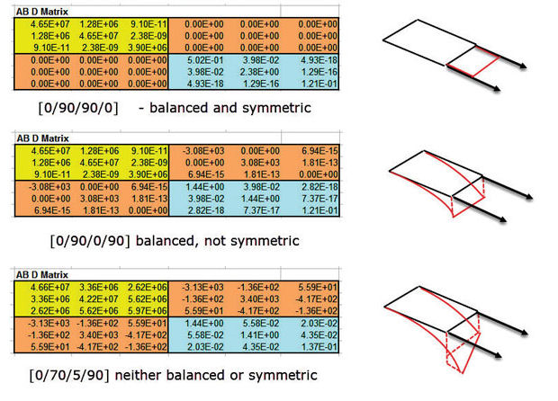 Fig. 9: Variations on balanced and symmetric plies in a laminate under axial loading.
The B matrix is the final matrix that is calculated. It indicates the coupling between in-plane loading and bending response, and is probably the most dominant term in design. If a pre-preg sheet is to remain flat after curing in an autoclave, the B matrix must be forced to decouple by only allowing symmetric plies.
Fig. 9 shows a range of possibilities with balanced and symmetric plies. The full ABD matrix array is shown.
Failure Prediction
Progressive ply failure assumes the stiffness of the failed ply can be reduced in some manner, and the analysis continued. Ply failures can continue to occur with subsequent reduction in stiffness.
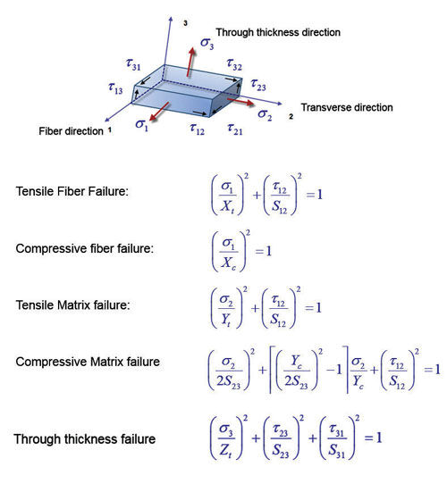 Fig. 10: Hashin-Rotem failure terms.
A progressive ply failure strategy requires:
- a failure criteria that can identify the mode of failure (Hashin, Puck, LaRC02, etc.); and
- a logical strategy for reducing element stiffness based on the mode of failure seen.
The Tsai-Wu failure theory described in Part I (DE, October 2014) is just one of many that were developed using known failure points and then interpolating in stress space using quadratic relationships. One of the limitations of this approach is that, although it is easy to program, all failure is based on a full and continuous interaction between stress states. It has been found experimentally that failure modes tend to be dominated by either fiber failure modes or matrix failure. There may be little interaction between them.
A class of failure theories has evolved that is sometimes described as “phenomenological,” to indicate the nature of the failure is implicit in the theory. These fit well with the progressive ply failure methods, as they indicate the type of strategy that should be followed in reducing stiffness caused by damage.
Transverse compression is interesting, because the strength is generally higher than transverse tension. The matrix tends to act to stabilize the fibers until some form of shear cracking occurs. If in-plane shear or longitudinal compression is present, this will also affect the way the ply behaves. This behavior is not well understood in general, and is the subject of much manipulation of the failure theories. Hashin-Rotem failure criteria breaks up the assessment of failure into several sub-criterion, any one of which can give a critical failure index:
- tensile fiber failure
- compressive fiber failure
- tensile matrix failure
- compressive matrix failure
- through thickness failure
Other Failure Models: Delamination
Two other FEA methods predict failure at the macro level:
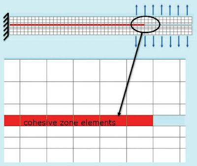 Fig. 11: Cohesive zone elements.
Cohesive element methods aim to model specific de-bonding or delamination situations by inserting a layer of special elements between the plies or materials, as shown in Fig. 11. The behavior of the crack or delamination front is controlled by an energy rate law to allow tuning for different types material (such as brittle or ductile). The actual damage method is still using a stress-based approach, relating stress state to resultant strain across the delamination. Optionally, separation or erosion of the elements can occur. Implementations vary from continuous 2D or 3D elements forming the cohesive layer, to simple springs exhibiting the stress strain behavior.
- An alternative to using stress-based delamination methods is to use fracture mechanics, postulating a crack at the ply boundary. The energy required to create new crack length or delamination zone forms a strain energy release rate. The force and displacements are known in the FEA model of an open crack, adjacent to the crack tip. Thus the energy required to oppose this and close the crack is also known. This is equal to the energy required to produce the delamination or crack. The method is commonly known as the Virtual Crack Closure Technique (VCCT), as shown in Fig. 12. The big advantage of the method is that the near singular stresses at the crack tip do not have to be evaluated.
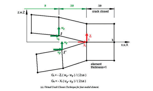 Fig. 12: VCCT operating at crack tip. Reference: Experimental-Numerical Investigation of Delamination Buckling and Growth. R. Kruger, C. Hansel, M. Konig. ISD-Report 96/3, November 1996.
The rate of change of energy with respect to the crack growth rate is analogous to the stress intensity factor in isotropic materials. The strain energy release rate can be compared to the fracture toughness of the material to establish whether a crack will propagate. The original implementations required a regular-sized mesh; advances now allow an arbitrary mesh.
In both methods, the crack will follow the mesh shape no matter what, so take care to avoid “forcing” the crack. A very fine mesh with no directional bias is best.
Micromechanics
In micromechanics, the composite material is assumed heterogeneous, rather than homogeneous as in macromechanics. Fiber and matrix are treated distinctly. The general terminology for “fiber” is broadened to “inclusion,” to allow for a variety of reinforcing media such as lamella (long fiber), ellipsoidal (short fiber) and spherical (beads, etc.). The inclusion is dispersed into a continuous “phase’ (the matrix). The microanalysis methodology includes classical solutions and FEA solutions.
The main objective is overall design and analysis of components and structures, using a more versatile range of micro-level stiffness and failure modeling techniques. Typical micromechanics methods assume a representative volume element (RVE) characterizes the extremely local effects. These can be integrated into a macro-level response to provide a form of progressive ply failure model. Fig. 13 shows a schematic of a typical macro-to-micro integrated approach.
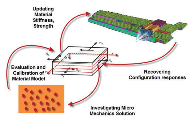 Fig. 13: Integrated micro- and macro-level approaches.
Macro level methods for predicting undamaged stiffness for thin plates and shells are well established. Strength prediction is still a challenge in many stress states, but it does seem that the more modern methods are more able to adapt to known experimental behavior.
The extreme example of this is in the relatively new usage in FEA of micromechanics methods. However, tight correlation with known experimental evidence is required, as more reliance is placed on advanced failure methods.
The decision on what level of technology to use should be based on a sensible assessment of the degree of safety margin required, the available test correlation evidence and proven experience with a particular method. For preliminary sizing, the use of simple macro-strain-based criteria is still probably most effective.
Subscribe to our FREE magazine, FREE email newsletters or both!
About the Author
Tony Abbey is a consultant analyst with his own company, FETraining. He also works as training manager for NAFEMS, responsible for developing and implementing training classes, including e-learning classes. Send e-mail about this article to [email protected].
Follow DE

