

Latest News
February 1, 2014
By Tony Abbey
Editor’s Note: Tony Abbey teaches live NAFEMS FEA classes in the US, Europe and Asia. He also teaches NAFEMS e-learning classes globally. Contact [email protected] for details.
One of the first things to appreciate about loading in finite element analysis (FEA) is that all loading is applied through the nodes in the model mesh. When using a modern graphical user interface in a preprocessor this might not be obvious, as in most cases we will be applying load to geometric entities such as surfaces and solid faces.
Functionality in the preprocessor allows nodes present in the mesh to be associated with the geometric surface or face. If we remesh to achieve a finer mesh, for example, the old nodes are deleted but the new nodes are associated with the surface or face—and hence to any loading that is applied.
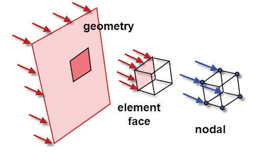 Fig 1: Loading hierarchy, from geometry to node. |
We can also apply loads directly to the faces of elements in a preprocessor; however, behind the scenes the solver is converting that element loading to an equivalent nodal loading. Fig. 1 shows schematically this chain of events.
A good example of the solver translation from element base loading to nodal-based loading is seen in a bar element. It is quite possible to apply either a distributed loading or midpoint loading to the bar. These forms of loading are converted by the solver to equivalent nodal point forces. Fig. 2 shows the simple equivalent nodal loading in a bar with a midpoint load.
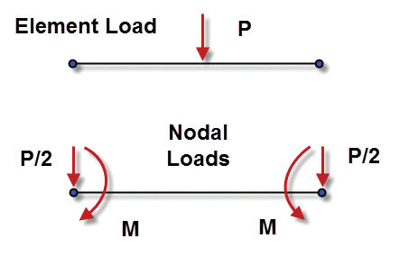 Fig 2: Equivalent nodal loads. |
The relationship between the implied element loading distribution and the nodal loading is quite subtle, as the goal is to produce what is called equivalent kinematic loading. This means that the element internal deflections defined by its shape functions, multiplied by the distributed loading, must balance the nodal deflections and equivalent nodal forces. In other words, work done must be in balance.
For simple element shapes and loading distributions, we could work this out by hand and apply equivalent nodal forces. However, with variable loading distributions and shapes, this calculation gets horribly complex—and quite unusual nodal point force values are required. For this reason, it is recommended that we always use distributed loading forms such as pressure, rather than trying to calculate nodal point forces.
Loading Types
The main types of mechanical loading that we can apply are pressures, defined by a scalar value and assumed acting normal to the element face or tractions that are applied as a vector. Fig. 3 shows the difference. We can also apply line loads and point loads. However, these are not recommended (as I will explain).
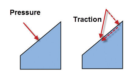 Fig 3: Pressure and traction on a surface. |
We can also apply body loads. In this case, we do not have to apply loading to individual entities; instead we define a loading environment that will be applied to the whole model.
The two main examples of this are inertia loading (sometimes called gravity loading) and centrifugal loading. In both cases, material density must be defined. Every element in the model will have a volume, and hence a mass. If the model is subjected to 10G acceleration in the vertical direction, for example, then each element will see a net force equal to its mass times 10G acceleration. This is distributed to each node in the element by the solver—so we end up with a sea of nodal point forces distributed throughout the structure.
For centrifugal loading, we need to define a spin axis and rotation speed. Each element again has its own mass, and also its offset from the spin axis. With this data, the solver can calculate the centrifugal force that each element sees—and again we end up with a distribution of nodal point forces throughout the structure. Fig. 4 shows typical inertia and centrifugal loading cases.
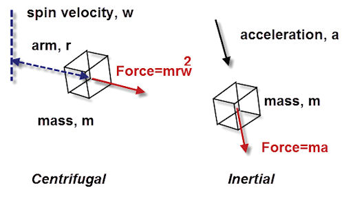 Fig 4: Inertial and centrifugal body loading. |
The final important class of loading is thermal loading. The heat flux passing through a surface can be defined. This requires that the topology of the surface is defined, which makes the data construct a little bit more awkward. However, in most preprocessors, this is hidden from the user. It is analogous to the topology definition required for a contact surface.
There are several other ways to define the thermal environment that are not strictly loading, but are more analogous to boundary conditions. These include temperature distributions, and convection and radiation conditions on external surfaces.
For linear and nonlinear static analysis, each of these loading distributions is assumed fixed in space. In dynamic analysis, using a transient approach, any of the loadings can vary through time. This applies to both linear and nonlinear transient dynamic analysis. A preprocessor will typically link a spatial distribution to a time history defined by a function or table input.
For a frequency-based dynamic analysis, loading can also vary as a function of frequency. We can input the magnitude of the loading in a similar way to a transient or time-based dynamic analysis. However, there may well be loading phase differences occurring as a function of frequency—and also spatially across the model at each particular frequency. This is something to plan carefully in advance, as it is easy to make mistakes.
Avoid Point Loads
For some applications, it is tempting to apply all of the external load at a single point. The bottom image in Fig. 5, for example, shows a bridge deck with a large force applied vertically because of a construction crane and its payload. Knowing the thrust line and the value of the force, it is easy to set up a point load. However, there are two main reasons why we should avoid doing this.
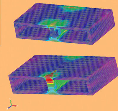 Fig 5: Bridge deck loaded with distributed load (top) and point load (bottom). |
1. If we apply a point load to a node, then we are applying a finite force value over an infinitely small area. The stress at this point is infinite. Think of a very narrow stiletto heel: The stress at the tip is high, and even with modest “ loading,” any thin aluminum or plywood sheet can be easily punctured. If we increase the mesh density in this area, the stress will keep going up. It is a stress singularity point. It may be that the point load represents the loading distribution into the structure quite badly, as shown in Fig. 5. This may mean that the region under the point of application sees unrealistically high stresses in the FEA model. Strengthening to deal with these may result in an overly conservative design.
2. Conversely, regions away from the point application may not see the correct load distribution—and in essence may be bypassed. The danger here would be a non-conservative design.
The goal is to assess how load is actually transferred into the structure and what that footprint looks like. Then imprint this onto the geometry so the mesh follows the shape. A distributed pressure can be applied as shown in the top image of Fig. 5.
It is essential to carefully assess the line of action of any externally applied load. Offsets will create moments and forces. Offset moments are a typical cause of high stress regions in structures.
Mapping from External Data
In many cases, pressure distribution applied to a structural surface is calculated externally. This may be a simple hand calculation of wind loading, for example, or it may be a full computational fluid dynamics (CFD) calculation. In both cases, the external data must be mapped to the structural mesh.
There are various ways this can be done; some multidiscipline solvers will allow direct mapping of a CFD pressure distribution to a structural mesh. The CFD data points are almost certainly going to be different from the nodal points in the structural mesh, and an interpolation is required. Alternatively, you may have to convert the externally calculated pressure distribution into an equivalent field or function definition in the preprocessor.
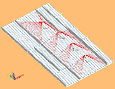 Fig 6: Helicopter floor pan loaded with spider elements. |
For the most accurate interpolation, the mesh density or data point distribution should be very similar between the CFD data and structural model. Ideally, the points will be spatially identical. In all cases, extrapolation should be avoided as it often results in highly inaccurate representations. The pressure distributions should be compared graphically, and also the net thrust and line of action should match.
Realistic Loading
I have mentioned that point loads are almost always going to be inappropriate to represent how load gets into a structure. But there are other examples where we need to consider how the loading will actually be distributed into our structural simulation.
For example, we may simplify a bolted connection with many discrete loading points into an equivalent pressure distribution. If we are not interested in local stresses in the connection region, then this is a good approach. A subtler example occurs where a thin-walled structure is loaded with a distributed pressure. In this case, the structure sees significant deformation—and we need to apply geometric nonlinear analysis to ensure that the induced membrane loading is modeled properly.
If we have a pin-bearing loading in a hole, for example, the traditional way of representing this is via a cosine pressure distribution acting normal to the bearing face over 180 °. In practice, with passing load or interference fit present, the loading distribution may be very different from this—and it may require a nonlinear contact analysis for accuracy.
Assume we have calculated the load applied to a flange from an abutting component. We know neither the pressure distribution nor the line of action. These should be set up to be conservative, with an upper value for the resultant movement arm between the line of action of the load and the shoulder of the flange.
Alternative Loading Methods
A convenient alternative to an applied pressure distribution is to input the loading via a spider type element. An example is shown in Fig. 6, where vertical inertial loading from passengers and seats is applied to the floor pan of a helicopter. Configuration changes can be easily set up, just by changing the point force values.
In this case, the spider type element is defined as a flexible or pure load distribution type. The important thing here is the spider itself contributes no stiffness to the structure. For airframe analysis like this, it is essential that the secondary seat structure stiffness does not add to the primary floor structure stiffness.
Conversely when applying torsion or moment to shafts, beams and similar structures, a rigid type spider element may be more appropriate. A point moment or torque is easily applied to the master node of the spider.
One final consideration is whether to apply displacements instead of forces to represent boundary loadings. In static nonlinear analysis, a displacement controlled loading will maintain stability more easily than force controlled loading in a structure that is softening from plasticity or buckling. In global-local modeling, displacement boundary conditions from the global model applied to the local model may deal better with mesh interpolation issues—or unrealistic local deflections.
There are many ways of applying loading. The objective should be to look at the real world loading and understand its transfer path into the structure. We want to model this as realistically as possible while staying conservative where we are uncertain of loading distributions or line of action.
Tony Abbey is a consultant analyst with his own company, FETraining. He also works as training manager for NAFEMS, responsible for developing and implementing training classes, including a wide range of e-learning classes. Send e-mail about this article to [email protected].
Subscribe to our FREE magazine, FREE email newsletters or both!
Latest News
About the Author
Tony Abbey is a consultant analyst with his own company, FETraining. He also works as training manager for NAFEMS, responsible for developing and implementing training classes, including e-learning classes. Send e-mail about this article to [email protected].
Follow DE

