Fig. 6: 3-2-1 constraint system applied to the crank.


February 1, 2015
Editor’s Note: Tony Abbey teaches live NAFEMS FEA classes in the US, Europe and Asia. He also teaches NAFEMS e-learning classes globally. Contact [email protected] for details.
Last month we looked at difficulties with boundary conditions when setting up a realistic FEA (finite element analysis) model. The three basic options are shown again in Fig. 1. The conclusions were:
• Defining equivalent pressure distributions as in Method 1A can ensure conservative loading is applied. Upper and lower bound variations can be used.
• Applying ‘hard’ constraints as in Method 1B produces singularities at the edge of the constraints that will disrupt the FEA stress results. Constraints tend to over stiffen the structure.
• General contact and glued contact methods as in Method 1C rely on the FEA method producing realistic and conservative bearing footprints.
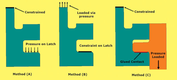 Fig. 1: Loading and constraint methods.
We are aiming for loading that has adequate moment offset to cater for uncertainties in the line of loading action. For instance, it may be better to imagine a triangular pressure distribution footprint in 1A so that the net force line offset is 2/3 of the latch width and not 1/2 of latch width. Fig. 2 shows these options.
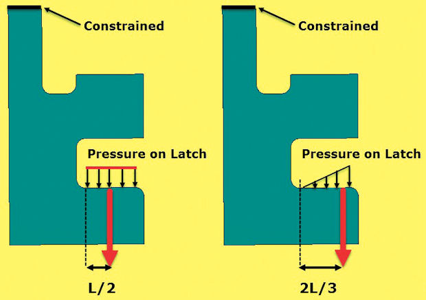 Fig. 2: Net force line variations.
This month we look at the extreme approach to applying equivalent pressure distributions throughout a structure to achieve balance, avoiding any direct constraint boundary modeling and rigid body motion. This powerful technique is the best way of setting up some FEA models.
The Scuba Tank Conundrum
Imagine you are tasked to carry out an FE analysis of a scuba tank. The loading represents no problem; an internal pressure, with external ambient pressure ignored. Similarly, the meshing and material definitions are straightforward. The objective is to check the stress concentrations around the nozzle and corner of the base.
The problem is—how do we constrain the model? We cannot run a static FE analysis with just a load balance, we need a constraint set that will remove all rigid body motion and ground the structure properly. The February 2014 Desktop Engineering article; “Accuracy and Checking Part 2” discussed checking for erroneous Rigid Body Modes (RBMs).
In reality, the scuba tank does not need external constraints, but the FEA will not work without them! Throughout my career, this was known as the “skyhook problem.” We need a skyhook that will ground the model, but not introduce unwanted load paths and incorrect stress distributions. Welding the base by constraining it to the ground will introduce over stiffening of the base. Only the local nozzle area will have a reasonable stress distribution. Similarly, “inventing” large grab handles and grounding them will introduce local stiffening in the walls and the stresses will be incorrect. The tank will not be free to expand radially between the grab handles.
The model should be grounded in a minimum way—but how? I have seen ship models welded to concrete waves and whole aircraft models propped up with tortuous beams and springs!
There is an elegant way to achieve the ‘skyhook’ – it’s called the 3-2-1 method.
The 3-2-1 Method
The 3-2-1 technique, applied to a full component without symmetry, uses three nodes. The nodes should be well spaced and orientated carefully as described.
• Fig. 3A: The first node has all three translational degrees of freedom (DOF) constrained. That gets rid of the three translational RBMs, but leaves the three rotational RBMs.
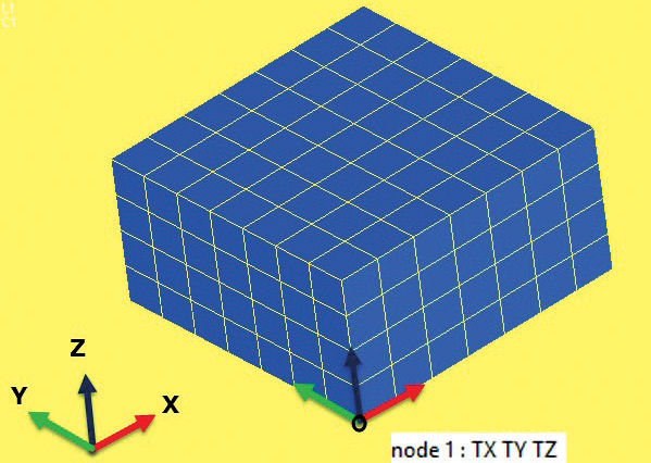 Fig. 3A: First Node
• Fig. 3B: The second node is positioned. Imagine a line connecting node 1 to 2. Node 2 has two translational DOF constrained in the two directions which are normal to this line. That gets rid of two rotational RBMs, but not the RBM “spinning” about the line. It has also allowed relative translational displacement to exist along the line node 1 to node 2.
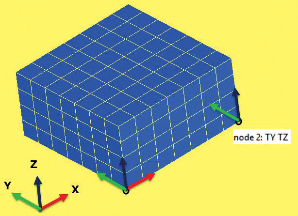 Fig. 3B: Second Node
• Fig. 3C: The third node is positioned and a single DOF is constrained normal to the plane of nodes 1, 2 and 3. This eliminates the final spinning RBM. This also allows relative translational displacement between any of the three nodes.
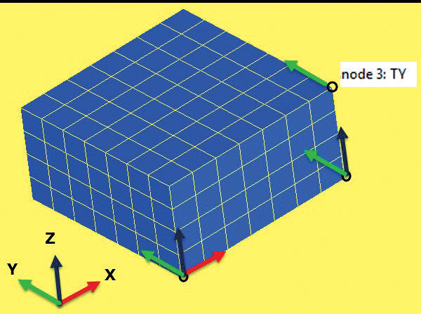 Fig. 3C: Third Node
If we now apply a balanced pressure load to the YZ plane faces, then a constant stress state is created and no local stress raisers occur (Fig. 4). The constraint reactions each become zero. This is an important point as it allows proper constraint of the model, but does not introduce any “external” constraint reactions.
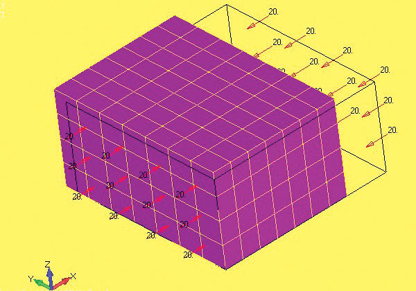 Fig. 4: Constant stress on deformed shape.
An Example of the 3-2-1 Method
Fig. 5 shows an actuator crank. Vertical load of 100 lbf is applied to the flat surface, creating a moment about the pivot point. The vertical load is reacted by the pivot bearing. The moment created is reacted by a couple consisting of horizontal 125.67 lbf forces between the pivot point and actuator rod attachment point. This is typical free body diagram used to check the force balance in the system. Do a quick check yourself by making sure the vertical forces, horizontal forces and moment about the pivot all balance.
It is essential that the applied loads balance as closely as possible. If there are any out of balance, then we create a net reaction force at the constraints. These reactions will cause enormous local stresses (each will become a stress singularity) and will wreck the model.
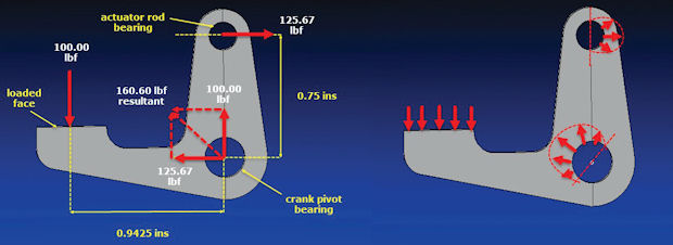 Fig. 5: Applied load balance on the actuator crank.
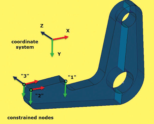
After balancing the load, we apply the 3-2-1 constraints. Fig. 6 shows the system chosen for the crank. There are many convenient combinations of three nodes we could have chosen; a set of three in a planar face is always a good starting point. If no convenient nodes exist you will have to create suitable locations. Slicing the geometry to create vertices where nodes will be generated is a powerful method. Be careful to get the relative node positions accurate as any small offsets or misalignment of the 3-2-1 system will cause reaction imbalances with huge local stresses.
The result of the FE analysis of the crank is shown in Fig. 7. The peak Von Mises stress is 69,437 psi. The location is at the inner transition radius. Stress vector plots confirm the peak local stress is a tensile stress tangent to the surface as expected. Material is steel with a yield stress of 215,000 psi, so the design is adequate.
In checking this analysis, we need to make sure the loading has been applied appropriately and accurately. A full report would include loading breakdown, loading assumptions and supporting FEA pre-processor model plots to show where the loading was applied.
The vertical applied load shown in Fig. 5 is assumed distributed over the rectangular face. However, we could be more conservative and assume a line of action closer to the free edge, giving a larger moment arm. This was tried out with line of action at 25% of surface length versus original 50%, and new balancing forces calculated. The peak local stress is now 77,748 psi, which is acceptable.
 Fig. 6: 3-2-1 constraint system applied to the crank.
The pivot bearing reaction force and line of action has been calculated as shown in Fig. 5. This is applied as a bearing distribution over an arc of 180° about the line of action. Care is needed here to make sure the correct line of action is used and that the loading does properly conform to the required distribution. If checking an analysis, evidence is needed. A typical assumption would be a sine distribution of normal pressure, with the peak value aligned along the 90° line. There are other empirical distributions you could use and many FEA pre-processors have these ‘hard-wired’, together with methods for defining line of action and distribution angle, which is a great convenience.
The actuator attachment bearing point is treated similarly. The assumption here is that the line of action is horizontal. A small error of 5° raises the peak stress only to 69,573 psi, so it is not that critical. However, sensitivities should be checked to make sure they are low.
If the actuator angle is significantly different then the load balance and stresses will change.
Indeed it would be possible to include this component in an independent kinematic analysis using a Multi Body Dynamics System (MBDS) tool. A range of reaction force sets could then be calculated as part of a full assessment of an operational cycle. Each reaction set from the MBDS analysis could then be applied as an independent load set in a 3-2-1 constrained FEA model.
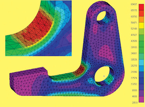 Fig. 7:Von Mises stress distribution of the crank.
Some FEA solvers can automate the connection of a component such as the crank, to a rigid link representation of the rest of an assembly. In normal usage the connection points are constrained to the rigid links. However it would be possible to recover the balancing forces, and use these to apply to an independent FE analysis using the 3-2-1 method.
The 3-2-1 relies on the provision of an accurate and realistic load balance. If the loading is not in balance, the model will wreck itself. If the loading distribution is not thought out it can become unrepresentative of the real world scenario.
If the loading becomes complex, this is probably the limiting factor on whether it is convenient to use the method. If the crank loaded face is offset, then out of plane moment is created which must be reacted through the two pins. This becomes awkward to represent as an equivalent bearing loading. Similarly if the pins are tapered, calculating reactions and mapping to equivalent pressure loading gets tricky. My advice would be to drop this method if the loading balance becomes difficult to calculate.
The set of three nodes should be widely spread to avoid large local couples and should avoid highly flexible parts of the structure (don’t use a node on a whip antenna!). The positioning of the nodes relative to each other must be accurate. The stiffness of adjacent components is ignored, such as the connecting pins in the crank arm. The influence of this should be assessed.
Geometric nonlinear analysis can’t be used with this method as the configuration and the load balance can change. The constraints will start to pick up non-zero reactions as the balance changes. However, material non-linearity and contact should be possible, but the method may introduce stability issues.
Subscribe to our FREE magazine, FREE email newsletters or both!
About the Author
Tony Abbey is a consultant analyst with his own company, FETraining. He also works as training manager for NAFEMS, responsible for developing and implementing training classes, including e-learning classes. Send e-mail about this article to [email protected].
Follow DE

