GPU Programming in MATLAB
The graphics processing unit promises higher computational performance.


Latest News
March 1, 2012
By Jill Reese and Sarah Zaranek
Originally used to accelerate graphics rendering, graphics processing units (GPUs) are increasingly applied to scientific calculations. Unlike a traditional CPU, which includes no more than a handful of cores, a GPU has a massively parallel array of integer and floating-point processors, as well as dedicated, high-speed memory. A typical GPU comprises hundreds of these smaller processors.
The greatly increased throughput made possible by a GPU, however, comes at a cost. First, memory access becomes a much more likely bottleneck for your calculations. Data must be sent from the CPU to the GPU before calculation, and then retrieved from it afterward. Because a GPU is attached to the host CPU via the PCI Express bus, the memory access is slower than with a traditional CPU. This means that your overall computational speedup is limited by the amount of data transfer that occurs in your algorithm.
Programming for GPUs in C or Fortran requires a different mental model and skill set that can be difficult and time-consuming to acquire. In addition, you must spend time fine-tuning your code for your specific GPU to optimize applications for peak performance.
This article demonstrates features in Parallel Computing Toolbox that enable you to run your MATLAB code on a GPU by making a few changes to your code. We illustrate this approach by solving a second-order wave equation using spectral methods.
Why Parallelize a Wave Equation Solver?
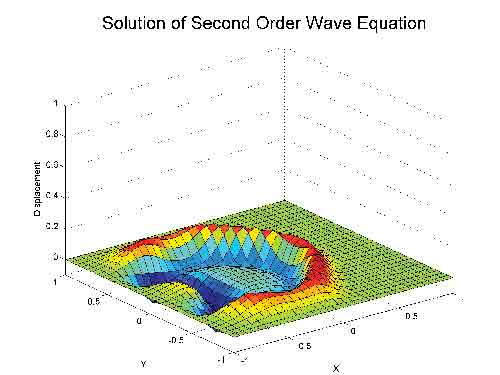 Figure 1: A solution for a second-order wave equation on a 32x32 grid. See animation here. |
Wave equations are used in a wide range of engineering disciplines, including seismology, fluid dynamics, acoustics and electromagnetics, to describe sound, light and fluid waves.
An algorithm that uses spectral methods to solve wave equations is a good candidate for parallelization, because it meets both of the criteria for acceleration using the GPU:
1. It is massively parallel. The parallel fast Fourier transform (FFT) algorithm is designed to “divide and conquer,” so that a similar task is performed repeatedly on different data. Additionally, the algorithm requires substantial communication between processing threads and plenty of memory bandwidth. The inverse fast Fourier transform (IFFT) can similarly be run in parallel.
2. It is computationally intensive. The algorithm performs many FFTs and IFFTs. The exact number depends on the size of the grid and the number of time steps included in the simulation (see Figure 1). Each time step requires two FFTs and four IFFTs on different matrices, and a single computation can involve hundreds of thousands of time steps.
Applications that do not satisfy these criteria might actually run slower on a GPU than on a CPU.
GPU Computing in MATLAB
Before continuing with the wave equation example, let’s quickly review how MATLAB works with the GPU.
GPU Glossary
|
FFT, IFFT and linear algebraic operations are among more than 100 built-in MATLAB functions that can be executed directly on the GPU by providing an input argument of the type GPUArray, a special array type provided by Parallel Computing Toolbox. These GPU-enabled functions are overloaded—in other words, they operate differently depending on the data type of the arguments passed to them.
For example, the following code uses an FFT algorithm to find the discrete Fourier transform (DFT) of a vector of pseudorandom numbers on the CPU:
A = rand(2^16,1);
B = fft (A);
To perform the same operation on the GPU, we first use the gpuArray command to transfer data from the MATLAB workspace to device memory. Then we can run fft, which is one of the overloaded functions on that data:
A = gpuArray(rand(2^16,1));
B = fft (A);
The fft operation is executed on the GPU rather than the CPU because its input (a GPUArray) is held on the GPU.
The result, B, is stored on the GPU. However, it is still visible in the MATLAB workspace. By running class(B),we can see that it is a GPUArray:
class(B)
ans =
parallel.gpu.GPUArray
We can continue to manipulate B on the device using GPU-enabled functions. For example, to visualize our results, the plot command automatically works on GPUArrays:
plot(B);
To return the data back to the local MATLAB workspace, you can use the gather command; for example:
C = gather(B);
C is now a double in MATLAB and can be operated on by any of the MATLAB functions that work on doubles.
In this simple example, the time saved by executing a single FFT function is often less than the time spent transferring the vector from the MATLAB workspace to the device memory. This is generally true, but is dependent on your hardware and size of the array. Data transfer overhead can become so significant that it degrades the application’s overall performance, especially if you repeatedly exchange data between the CPU and GPU to execute relatively few computationally intensive operations. It is more efficient to perform several operations on the data while it is on the GPU, bringing the data back to the CPU only when required.
Note that GPUs, like CPUs, have finite memories. However, unlike CPUs, they do not have the ability to swap memory to and from disk. Thus, you must verify that the data you want to keep on the GPU does not exceed its memory limits—particularly when you are working with large matrices. By running gpuDevice, you can query your GPU card, obtaining information such as name, total memory and available memory.
Implementing and Accelerating the Algorithm
To put the above example into context, let’s implement the GPU functionality on a real problem. Our computational goal is to solve the second-order wave equation, with the condition u = 0 on the boundaries:
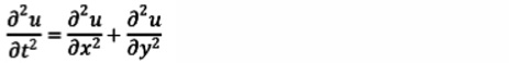
We use an algorithm based on spectral methods to solve the equation in space, and a second-order central finite difference method to solve the equation in time.
Spectral methods are commonly used to solve partial differential equations. With spectral methods, the solution is approximated as a linear combination of continuous basis functions, such as sines and cosines. In this case, we apply the Chebyshev spectral method, which uses Chebyshev polynomials as the basis functions.
At every time step, we calculate the second derivative of the current solution in both the x and y dimensions using the Chebyshev spectral method. Using these derivatives together with the old solution and the current solution, we apply a second-order central difference method (also known as the leapfrog method) to calculate the new solution. We choose a time step that maintains the stability of this leapfrog method.
The MATLAB algorithm is computationally intensive, and as the number of elements in the grid over which we compute the solution grows, the time the algorithm takes to execute increases dramatically. When executed on a single CPU using a 2048x2048 grid, it takes more than a minute to complete just 50 time steps. Note that this time already includes the performance benefit of the inherent multithreading in MATLAB. Since R2007a, MATLAB supports multithreaded computation for a number of functions. These functions automatically execute on multiple threads without the need to explicitly specify commands to create threads in your code.
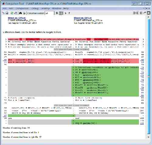 Figure 2: The Code Comparison Tool shows the differencesin the CPU and GPU versions of the code. The GPU and CPU versions share over 84% of their code in common (94 lines out of 111). |
When considering how to accelerate this computation using Parallel Computing Toolbox, we will focus on the code that performs computations for each time step. Figure 2 illustrates the changes required to get the algorithm running on the GPU. Note that the computations involve MATLAB operations for which GPU-enabled overloaded functions are available through Parallel Computing Toolbox. These operations include FFT and IFFT, matrix multiplication, and various element-wise operations. As a result, we do not need to change the algorithm in any way to execute it on a GPU. We simply transfer the data to the GPU using gpuArray before entering the loop that computes results at each time step.
After the computations are performed on the GPU, we transfer the results from the GPU to the CPU. Each variable referenced by the GPU-enabled functions must be created on the GPU or transferred to the GPU before it is used.
To convert one of the weights used for spectral differentiation to a GPUArray variable, we use:
W1T = gpuArray(W1T);
Certain types of arrays can be constructed directly on the GPU without our having to transfer them from the MATLAB workspace. For example, to create a matrix of zeros directly on the GPU, we use:
uxx = parallel.gpu.GPUArray.zeros(N+1,N+1);
We use the gather function to bring data back from the GPU; for example:
vvg = gather(vv);
Note that there is a single transfer of data to the GPU, followed by a single transfer of data from the GPU. All the computations for each time step are performed on the GPU.
Comparing CPU and GPU Execution Speeds
To evaluate the benefits of using the GPU to solve second-order wave equations, we ran a benchmark study in which we measured the amount of time the algorithm took to execute 50 time steps for grid sizes of 64, 128, 512, 1024, and 2048 on an Intel Xeon Processor X5650, and then using an NVIDIA Tesla C2050 GPU.
For a grid size of 2048, the algorithm shows a 7.5x decrease in compute time from more than a minute on the CPU to less than 10 seconds on the GPU (see Figure 3). The log scale plot shows that the CPU is actually faster for small grid sizes. As the technology evolves and matures, however, GPU solutions are increasingly able to handle smaller problems.
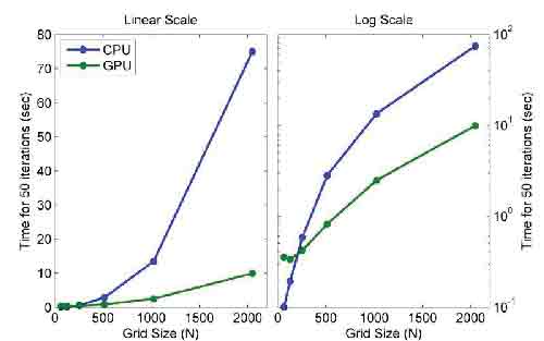 Figure 3: The linear scale plot (left) and log scale plot (right) of the same benchmarks results show the time required to complete 50 time steps at different grid sizes. |
Advanced GPU Programming with MATLAB
Parallel Computing Toolbox provides a way to speed up MATLAB code by executing it on a GPU. You can change the data type of a function’s input to take advantage of the MATLAB commands that have been overloaded for GPUArrays. A list of built-in MATLAB functions that support GPUArray is available in the Parallel Computing Toolbox documentation.
To accelerate an algorithm with multiple simple operations on a GPU, you can use arrayfun, which applies a function to each element of an array. Because arrayfun is a GPU-enabled function, you incur the memory transfer overhead only on the single call to arrayfun, not on each individual operation.
Finally, experienced programmers who write their own compute unified device architecture (CUDA) code can use the CUDAKernel interface in Parallel Computing Toolbox to integrate this code with MATLAB. The CUDAKernel interface enables even more fine-grained control to speed up portions of code that were performance bottlenecks. It creates a MATLAB object that provides access to your existing kernel compiled into PTX code (PTX is a low-level parallel thread execution instruction set). You then invoke the feval command to evaluate the kernel on the GPU, using MATLAB arrays as input and output.
Engineers and scientists are successfully employing GPU technology, originally intended for accelerating graphics rendering, to accelerate their discipline-specific calculations. With minimal effort and without extensive knowledge of GPUs, you can now use the promising power of GPUs with MATLAB. GPUArrays and GPU-enabled MATLAB functions help you speed up MATLAB operations without low-level CUDA programming. If you are already familiar with programming for GPUs, MATLAB also lets you integrate your existing CUDA kernels into MATLAB applications without requiring any additional C programming.
To achieve speedups with the GPUs, your application must satisfy some criteria, among them the fact that sending the data between the CPU and GPU must take less time than the performance gained by running on the GPU. If your application satisfies these criteria, it is a good candidate for the range of GPU functionality available with MATLAB.
Jill Reese is a senior software engineer and Sarah Zaranek does MATLAB product marketing at MathWorks. Contact them via [email protected].
MORE INFO
Subscribe to our FREE magazine, FREE email newsletters or both!
Latest News
About the Author
DE’s editors contribute news and new product announcements to Digital Engineering.
Press releases may be sent to them via [email protected].


