Impact, Drop and Crash Testing and Analysis
Impact analysis, virtual drop testing and virtual crash analysis are important finite element analysis tools in use throughout the vehicle, mobile phone, appliance and many other industries.


Latest News
August 1, 2013
Many companies have mature and well-understood techniques for simulating new products using such methods as impact analysis, virtual drop testing and virtual crash analysis. However, years of test and analysis correlation lie behind this. Companies new to the field now have user-friendly finite element analysis (FEA) tools, but the challenges of the fundamental engineering and simulation methods remain. Here are a few of the important areas to consider.
Impact Analysis
It is useful to consider vehicle impact speeds to describe the different physics involved and that we wish to simulate.
Consider a minor bump, such as overrunning a parking spot and hitting a lamppost. At around 5 mph, the resultant damage is not excessive. The hood may permanently buckle, and the front grille and bumper become dented. The simulation required here is relatively straightforward: We model the external contact between the lamppost and car, and also the internal contact between the car components. There may be as few as five or six.
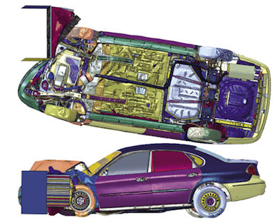 Fig. 1: Vehicle crash simulation. Image courtesy of Dassault Systèmes SIMULIA and NCAC. |
Clearly, we need nonlinear material and plasticity—the bumper and hood are permanently deformed. The low impact speed is not producing strain rate effects in the material. We can assume there is no fracture or tearing present in the components. It is a dynamic situation, where the inertia effects of the vehicle and components are important. This all adds up to a nonlinear transient solution with straightforward contact, large displacements and material plasticity.
Alternatively, imagine a Formula One car hitting a crash barrier at 200 mph. At this speed, the strain rate effects of the materials involved are significant.
Strain rate can be demonstrated by using a lump of plastic modeling clay: Pull slowly to get one form of deformation; pull fast to get a completely different response. A large and complicated deformation of the structure results, with components contacting in unpredictable ways. Fracture or tearing of components and failure of bolts, spot welds and bond lines will also occur.
This all adds up to a highly nonlinear transient solution with complex contact behavior, large displacements, material plasticity and strain rate effects and failure of components and connections.
Implicit and Explicit Solution Choice
An initial objective in our analysis of any drop, impact or crash scenario is to assess what level of physical simulation we have to use. The first choice we have to make when considering the simulation technique is whether to use an implicit or explicit solution. Both methods are mainstream FEA simulation techniques, but they are very different in their backgrounds and implementation.
The low-speed vehicle bump could well be analyzed using an implicit solution, thanks to the simplicity of the contact scenario, lack of strain rate effects or material failure. If we can use an implicit solution, there are some big advantages.
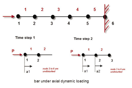 Fig. 2: Bar under axial loading, explicit approach. |
The high-speed crash, on the other hand, will require an explicit solution. Complex contact behavior, strain rate effects and component failure are all very much the forté of explicit solvers.
It is difficult to give an exact point at which we would migrate from an implicit to an explicit solver, but any object impact above 15 mph is probably in the explicit domain.
Implicit Solvers
FEA’s traditional definition implies the implicit solution. The structure is idealized by finite elements and the stiffness and the mass of each is calculated. The overall structural representation is then created by assembling all element stiffness and mass terms into one big system matrix for solution. Displacements at each of the connecting nodal points are calculated. Dynamic analysis differentiates the displacement through time to get velocities, and the velocities to get accelerations. At each time step, stresses and strains are derived from displacements.
We can characterize this type of solution “heavy lifting” up front to solve for the system equations, and then use those equations in the subsequent time history analysis.
Explicit Solvers
An explicit solution is set up in a similar way to the implicit solution. We can even share the mesh between the two solutions if needed. However, the underlying process is different. Instead of solving a set of very large system matrices, elements and connecting nodes are treated on an individual basis.
For example, Fig. 2 shows a simple rod impacted at one end. The first node in contact sees the force being applied; it has mass. By using Newton’s second law (force = mass x acceleration), we can calculate the acceleration. We can now calculate its velocity and displacement over a very brief time interval.
The first node will then impact the second node, transmitting a force and imparting acceleration. The acceleration, velocity and displacement of nodes 1 and 2 are updated—and so on. The fundamental calculation at each node is the acceleration. From this a velocity, and hence strain rate is derived. From this a strain, and hence stress is derived.
As mentioned above, we can characterize the explicit solution as needing no heavy lifting up front, but it does require a lot of housekeeping as we march forward. Accelerations are fundamental quantities, and strain rate effects are a key part of the process. Stresses and strains at a point in time require two lots of integration.
Advantages and Disadvantages
The big advantage of explicit solvers is that they handle highly nonlinear simulations required for many drop, impact and crash situations. In addition, complex material models are easily implemented. Without a fixed up-front system matrix calculation, the solution is very adaptable. Elements can be deleted from the solution, and tearing and fracture are easily modeled—as shown in Fig. 3.
The solution cost of the explicit model generally scales proportionally with size, in terms of number of elements or degrees of freedom. In the implicit solver, the solution cost is proportional to model size squared.
The disadvantages of an explicit solver include the time step size. This tends to be much smaller than the implicit solver, and is a function of the smallest element size and material density. We have to be cautious in modeling very fine detail: A tiny fillet, tooling hole or other unimportant feature can result in higher cost. Review the meshing strategy and the resultant mesh carefully.
Short events, with durations measured in milliseconds, are ideally suited for explicit analysis. Soft impact implies a long-duration event. If in the order of seconds, it can become a serious computational burden. A free-fall phase of a drop would never be modeled, for example. The object would be modeled in position, just prior to impact. The velocity and impact orientation must be carefully assessed. Rebounds are simulated by freezing the object so it has an inelastic response with rigid body mechanics.
Initial Loading State
Many impact events occur during operational loading conditions. For example, a bridge may have normal gravity and traffic loading at impact. We can’t just apply the normal loading at time zero, as dynamic analysis starts with a bang. Traffic and gravity loading is impulsively applied at time zero, giving a dynamic response.
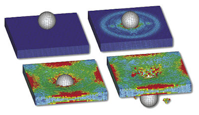 Fig. 3: Impactor penetrating through plate. Image courtesy of NEi Software |
Two approaches are used to avoid this. In the first, the static load is slowly applied, ramping up over a long time. System damping dissipates dynamic response. After stable static load distribution is achieved, impact loading can begin. Keep in mind, however, that it can take more resources to establish the static load distribution than to carry out the impact analysis.
An alternative uses implicit results from static loading of a common mesh. This is also ramped up to avoid dynamic response; however, it is often easier to use this approach. The tricky part is ensuring the stress and strain distribution is mapped accurately and appropriately to the explicit model.
Model Checking
An explicit solver is more versatile than an implicit solver because the large system matrices and cumbersome solution process are largely avoided. The main downside is that stability of the solution is not guaranteed.
Instability associated with element formulation results in hourglassing. This is an internal element mode that has no physical meaning. It can affect results and destroy the accuracy of the overall model. However, the energy associated with hourglassing can be plotted as a function of event time. Kinetic energy (due to motion) and potential energy (due to deformation) can also be plotted through time. The interchange of these energy forms—in total and on the component basis—are very valuable checks.
A checking technique for initial motion direction and contact orientation increases the density of all components by an arbitrary factor of, say, 100. This renders the analysis meaningless, but allows fast initial configuration verification because the time steps are 100 times bigger.
Checking will follow many aspects of implicit analysis, such as mesh distortion, cracks in the model, etc.
Data Output and Post-processing
An explicit solver has two streams of output. Full plot states are output sparingly to give an overall impression of the impact and subsequent behavior. XY plot data is typically a nodal or elemental result against time.
The nodes or elements have to be chosen up front, so it is important to review the model carefully and decide where this information will be most useful. This is a very good discipline, and is analogous to strain gauging. With good planning, a great deal of useful response information will be gathered.
Accelerations are a fundamental output; derived quantities such as displacement and stress are more approximate. In addition, the solution gives noisier output than an implicit solution. Responses are filtered to remove extraneous simulation noise. Stress contours will also be more ragged than implicit solutions. Care is needed with the interpretation of stress contours, etc., at a particular time step.
Predicting stress-based failure is complicated. The results are transient. It is a matter of interpretation whether sufficient energy has been absorbed by a bolt, for example, to cause actual rupture.
The uncertainties with filtering and failure prediction mean that comparative tests should always be made when using explicit analysis in a drop impact or crash scenario.
My recommendation when embarking on explicit analysis is to allow sufficient time to go up what can be a steep learning curve. Keeping in touch with reality is essential in what is a demanding level of simulation, so comparison with test or previous analysis should always be made.
Tony Abbey is a consultant analyst with his own company, FETraining. He also works as training manager for NAFEMS. Send e-mail about this article to [email protected].
More Info
Subscribe to our FREE magazine, FREE email newsletters or both!
Latest News
About the Author
Tony Abbey is a consultant analyst with his own company, FETraining. He also works as training manager for NAFEMS, responsible for developing and implementing training classes, including e-learning classes. Send e-mail about this article to [email protected].
Follow DE

