Figure 3. Modelling of a bolt using 3D elements and nonlinear contact


Latest News
May 5, 2014
Editor’s Note: Tony Abbey teaches live NAFEMS FEA classes in the US, Europe and Asia. He also teaches NAFEMS e-learning classes globally. Contact [email protected] for details. A Joints and Connectors class in FEA starts on July 1st. Click here for details.
Most structures involve some form of jointing or connection. Using rivets to connect structural plates is almost as old as the introduction of bronze and then iron into early civilization. Bolted connections became possible with the advent of screw cutting methods and usage was accelerated by the standardization of pitch and thread, for example. Even today, fabricated structures such as aircraft and ships use many thousands of bolts and rivets to connect components together. Other large-scale connection technologies include welding and spot welding. The improvement of adhesive technology coupled with much wider use of composites has meant a major resurgence in the use of bonding.
Connections can be of a continuous nature, such as in large surface regions of plates, flanges and where other abutments exist. Alternatively, discrete load paths may be formed by lugs and pins, clips or similar connectors.
The engineer is faced with a difficult decision when attempting to simulate such connections and joints within a finite element analysis (FEA). In many cases the details of each individual connection can be ignored if an overall stiffness or strength assessment is to be made and the connection is assumed reasonably continuous. However there may be doubts about the local flexibility and load paths developed with this assumption. It may be that the assessment of local behavior of the connector is essential to a safety case, for example with main attachment fittings. In some cases the interaction between the connectors and the surrounding structure is critical, as in the case of pre-loaded bolts and inter-rivet buckling.
This article looks at the various modeling assumptions and implications when considering bolted type connections. Other connections such as spot welds, continuous welds and bonding will be considered in a separate article.
Bolting Requirements
Figure 1 shows the main characteristics of a typical bolted joint. The bolt consists of a shank and a head. The end of the shank is threaded to accept the nut. There usually a washer underneath the nut and possibly also the bolt head. In some applications, the thread is allowed to extend into the grip length. The grip length is the part of the shank containing the plates, flanges or other components which are being connected. Most bolts are preloaded, which we will discuss in more detail shortly, and so one of the primary actions is to clamp the components together between washer faces or nut washer and head face. These two faces also constrain components from separating axially as a result of external forces applied to them.
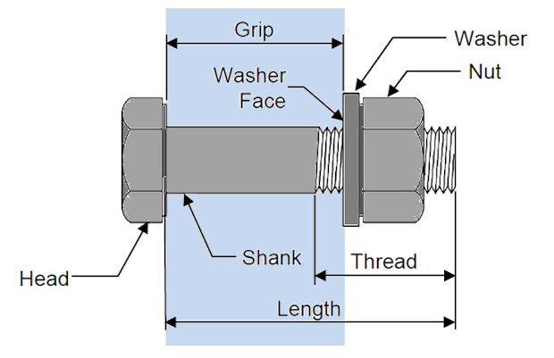 Figure 1. Bolt terminology
A typical tension load scenario is shown in Figure 2, together with a single-shear load scenario. An alternative to the single-shear can exist when there are three plates; this is called double-shear and is preferred as no offset moment occurs. In most industries, the shear load transfer path is by plate bearing loads causing shearing across the bolt shank. To balance the shears, particularly in single shear loading, complementary bending distribution occurs in the bolt shank and can also be reacted by contact of the components under the nut and head under high distortion. Some industries, such as civil engineering, require the load transfer via shear-only loading to occur through friction between heavily clamped components and bolt head and nut. A gap between bolt hole and shank and very high pretension loads are required to achieve this type of load transfer.
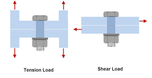 Figure 2. Bolt Tension and Shear loading conditions
FEA Simulation
The most intuitive form of FEA simulation is by using solid elements and nonlinear contact surfaces. If there are relatively few bolts in the system and CAD geometry of the bolt details is available, then this becomes a viable simulation method. We will look at other alternatives shortly.
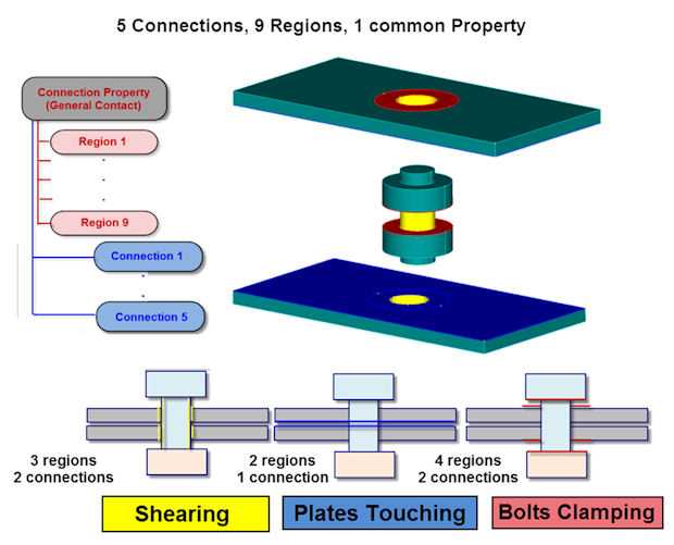
Figure 3 shows a typical setup of transferring load between two plates via a bolt. The simplified geometry is shown for clarity, rather than the FEA mesh. In particular we can see that the bolt head, shank, nut and washers have all been morphed into a single object. The effective stiffness of the combined bolt head and washer and combined bolt nut and washer have to be checked. There is no representation of the thread and we assume the three primary load transfer paths are as shown in the figure.
 Figure 3. Modelling of a bolt using 3D elements and nonlinear contact
The main challenge for this type of modeling is to make sure that the contacts are set up properly. Each contact consists of a pair of regions that are joined by a connector and have a connection property. Each contacting region is defined in the solver by a zone of element surface topology, however for ease of preparation we can usually define this via the parent geometry. The connectionis the definition of which region pairs are potentially in contact. The property defines the contact method; the contact could be glued (i.e. permanently locked shut), general nonlinear contact, or various other types. Other information such as friction and interference tolerances can also be defined.
When deciding whether to use this type of connector modeling, assess the ease with which contacts can be set up. Ideally the preprocessor or embedded CAD environment should be able to automatically detect potential contact surfaces and present these to the user in a highly visual manner. It should then be a straightforward housekeeping exercise to allocate connector properties and delete unwanted connections. If the implementation is labor-intensive, then it is probably a good idea to avoid this type of approach as the amount of data required in even a simple situation as shown in Figure 3 becomes unworkable.
Notice that in Figure 3 the three main load transfer paths have been idealized as shearing, plate touching and bolt clamping as shown with the inset figures. The plate touching zone is usually quite small and localized around the bolt. To extend the mutual contact between the plates over the complete plate surface is usually unnecessary and adds a lot of computational effort to the solution. It can also result in convergence problems. The plates can be tied together via normal springs in this zone if difficulty arises.
In a nonlinear analysis, various pitfalls arise including stability and convergence. During initial load steps of a nonlinear analysis a full load path is not achieved. This means that the bolts have an indeterminate solution and we may observe bolt spinning or chattering in position. Remedies include moving all bolts and components into initial bearing contact, by updating the CAD geometry, and preventing rigid body motion of the bolts by including very weak system springs. This is especially effective for spinning of bolts. The contact surface technology in the solver should be mature enough to fit a continuous smooth surface through the nodal points which form contact between the bolt and the bolt hole. This will smooth out any point loadings due to mesh discretization.
Bolt Preload
Most bolting systems involve a bolt preload. In the real world this is applied by torqueing the bolt against the nut and pre-stressing the shank. In an FEA simulation, it would be unusual to model the full thread engagement between the bolt and the nut. Very detailed 3D models that simulate this effect are possible, but they are extremely computationally expensive and pretension is very sensitive to correct friction properties and geometric accuracy.
The general principle of pretension is shown in Figure 4. The tensile bolt load creates a reactive compressive load between the components and the bolt head and nut. A common goal is to keep the components in compression under external loading, for example to improve fatigue life. One of the difficulties when calibrating this type of FE model is that hand calculation of the internal load balance when an external load is applied to the components is very difficult. Bolt load diagrams can be created, but they make simplistic assumptions about how the external load is transferred into the pre-stressed bolt, nut and component system. These diagrams can be very misleading and unrealistic. The best approach when attempting to validate an FEA pre-load system is to carry out simple test models such as clamping of a pair of back-to-back plates in pure tension or pure shear, similar to the loading actions shown in Figure 2.
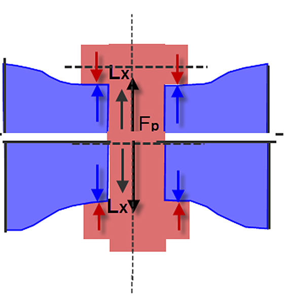 Figure 4. Bolt pre-load schematic.
There are several ways that the bolt preload can be introduced into an FEA model. One of the earliest approaches gives the bolt material a coefficient of thermal expansion, and the remainder of the model zero coefficient of thermal expansion. A thermal load case applies a temperature differential to the bolt material. This creates thermal strains which are used to simulate mechanical strains present in a preload. The temperature differential is tuned give the correct preload value. A more modern approach uses a dedicated bolt preload option such as shown in Figure 5. A datum plane splits the shank of the bolt. The datum plane can usually be defined either via pure geometry or by a group of nodes. A bolt axis is defined along which the preload will act. The elements or geometry containing the bolt head section and nut section are also defined. The preload is applied by various methods, including a constraint equation that literally pulls the two split services through each other to apply a pre-stress. Various options include allowing an initial preload, which remains constant throughout any external loading, or a preload which can be unloaded due to external forces applied to the components. The implication of these two options should be carefully checked with the test cases described earlier.
Various other forms of pre-loading are available in some solvers, including the so-called mesh-less bolt, where the bolt itself is not modeled but a balanced pressure load is applied to the footprint of the head and nut onto the facing components.
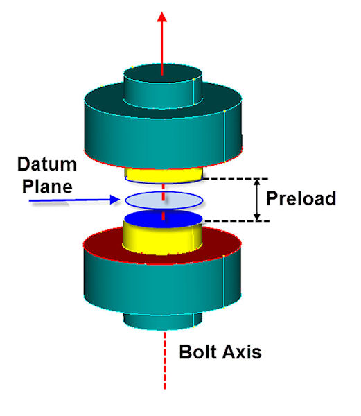 Figure 5. Bolt pre-load method in an FEA solution applied to parent geometry.
1D Bolt Modeling
If a large number of bolts are to be modeled, then the use of solid element representation can be far too burdensome in terms of setup time, contact complexity and computational cost. An alternative is to use a 1D beam element representation. This can also use a similar preload method. A typical example is shown in Figure 6. There are many different implementations of this approach, but we will focus on a method which uses a rigid element to spider out the head and nut tend of the bolt to the top and bottom plate respectively, and can connect to 2D or 3D element representation. The rigid element takes up the cross-sectional area of the bolt shank and distributes the load out to the periphery of the plate hole. This can be used in a linear analysis, which is another big advantage. However, the downside is that the load path in bearing between the bolt and the plate is incorrect as the back face is being pulled in tension. This can be improved by having a 180 degree spider aligned with the bearing surface. This does mean that the load path has to be accurately predicted so that it is aligned with the spider orientation and the bolt is still rigidly bonded into the plate over 180 degrees.
If a beam element is used to represent the bolt then the bolt bending and shear stiffness are reasonably representative. Some FEA implementations have a more advanced form of beam representation to model the very short stiff beam which a bolt represents. However, what is missing from this representation is the bearing stiffnesses of the plate and beam.
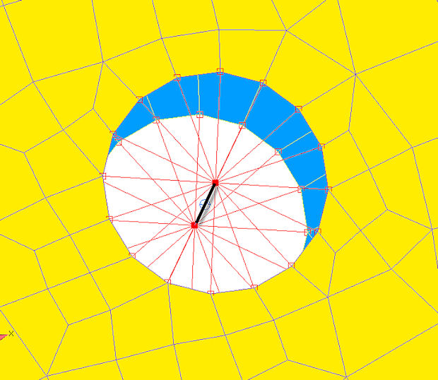 Figure 6. 1D bolt modelling method, shown here with 2D shells.
The stiffness is can be visualized by looking at Figure 7 which shows the deformation modes associated with the pin and the plates. We can put back the bearing stiffness by introducing springs between the top of the beam and the spider element. These springs can also be used to adjust the axial stiffness if required.
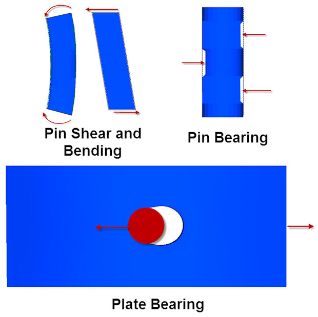 Figure 7. Deformation modes of bolt and plate.
Using this technique the stiffness of the joint can be modeled very effectively. However, as mentioned before, the local load transfer between the bolt and the plate is very inaccurate as the bolt is rigidly bonded to the hole. Although the stresses are locally quite poor, they do not dominate the overall stress distribution in the plate and the spurious local stress region can be ignored. Instead the bolt transfer loads are extracted from the analysis results and used in a post FEA solution for plate bearing strength assessment. This is a very well established process and does not warrant detailed FEA analysis. Similarly the strength of the bolt can be quickly assessed by knowing the forces and moments in the bolt. If these are extracted then very simple but effective hand calculations can be carried out as shown in Figure 8.
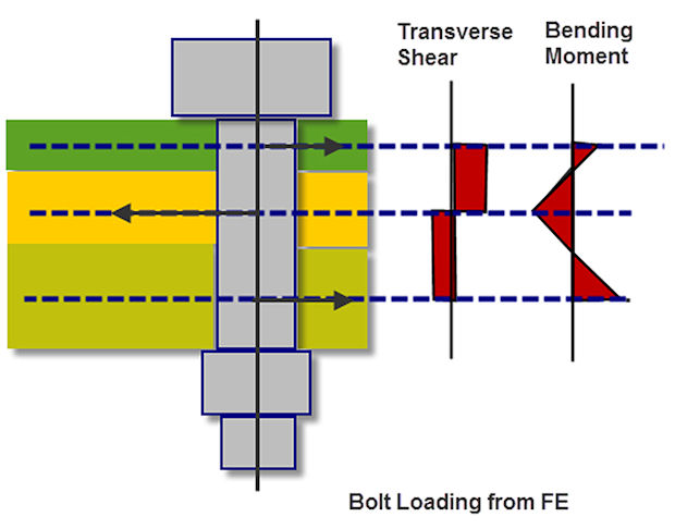 Figure 8. Bolt strengths assessed from FEA forces and moments.
However, what should be avoided is a point connection from the end of the beam into the plate that ignores the load distribution of the pin circumference. Figure 9 shows a stress contour plot of a plate loaded by several bolts where the load transfer is occurring at individual nodes. This is a situation where a finite force is transferred through an infinitely small area and creates a singularity at each connection. If we increase the mesh fidelity then we chase the singularity and the local stresses will ‘blow up.’ This can be awkward to explain in a report and should be avoided. It doesn’t take much effort to introduce the approach shown in Figure 3, with stresses shown in Figure 10. Although the stresses are not accurate, they do not dominate the loading in the plate.
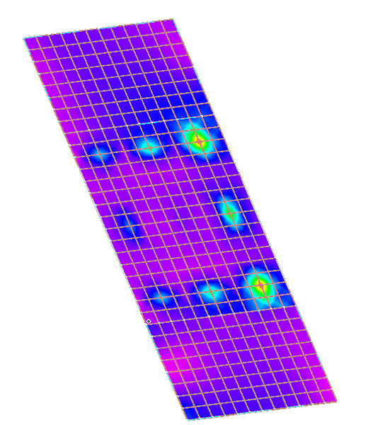 Figure 9. Poor local bolt connection modeling.
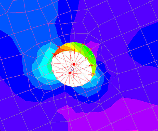 Figure 10. Recommended local bolt connection modeling.
Consider Your Objectives
Modelling of bolted joints needs careful consideration of the analysis’ objective. Are the bolts critical members which need individual modeling or can the load transfer path be adequately represented by 1D idealization? If strength assessment of multiple bolts is to be tackled, then consider using traditional post FEA calculations for bolt and plate strength.
The time needed to model bolts using nonlinear 3D contact may be prohibitive.
Pre-tension in bolts should always be checked using simple test models to understand the initial loading and stress distribution, and the subsequent redistribution under external loading.
Tony Abbey is a consultant analyst with his own company, FETraining. He also works as training manager for NAFEMS, responsible for developing and implementing training classes, including a wide range of e-learning classes.
Subscribe to our FREE magazine, FREE email newsletters or both!
Latest News
About the Author
Tony Abbey is a consultant analyst with his own company, FETraining. He also works as training manager for NAFEMS, responsible for developing and implementing training classes, including e-learning classes. Send e-mail about this article to [email protected].
Follow DE

