Fig. 1: Geometry, mesh and loading of a yoke structure.


Latest News
May 1, 2015
Editor’s Note: Tony Abbey teaches live NAFEMS FEA classes in the United States, Europe, and Asia. He also teaches NAFEMS e-learning classes globally. Contact [email protected] for more details.
There are two ways of solving response analysis: direct and modal methods. The direct method uses physical degrees of freedom (DOF) of the model. A structure modeled with 200,000 DOF has stiffness and mass matrices of this order. On the other hand, if we use a modal method then the DOF are represented by the number of modes — say 50. This reduces the size of the mass and stiffness matrices to this order. The computing cost of solving modal-based solutions is much cheaper than using a direct method. We can also reuse a modal database that reduces the cost even further.
However, as with all things, we don’t get something for nothing. The big danger in a modal method is reliance on finding all the modes needed to describe the dynamic response. In some cases, the number of modes can be very high and modes may be missed or difficult to calculate accurately. So, in general, the direct method is more accurate — but more expensive. In practice we will use both methods, rather than just focusing on one. A modal-based analysis can get us answers quickly and help us to understand the physics of the problem. A follow-on direct method can confirm the accuracy.
Please remember that whichever method you use, a physical understanding of the important modes in the structure is the key. The real structure will respond based on its inherent modal characteristics, so we should know as much about these as possible. You should always do a preliminary normal modes analysis, even if you are aiming for a direct transient analysis that does not strictly need them. This was stressed in the previous article and the sermon continues.
Transient Analysis Time Step
In real life, the structure will see a continuous response to any form of input loading. The finite element analysis (FEA) method discretizes this into a set of finite time steps. For many applications, this is a fixed-time step interval. The response through time is evaluated by a “time-marching” approach. The traditional FEA method solves for displacement, and so velocity and acceleration have to be estimated at each time step.
Force and displacement are “smeared” over three adjacent time points in this method. This has an important implication: If we make the time step too coarse, we will get very poor results. This leads us to our first practical point: What size of time step should we consider? We use the highest frequency of interest to us in the response analysis. To determine that will require engineering judgment, but we should have some clues available. It may be defined as an input specification, or equipment operating frequencies. If you are uncertain, use a safety factor of 1.5 or 2.0 on the upper value.
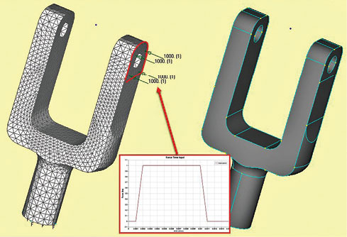
I am using the model shown in Fig. 1 to illustrate the methods in the article. This is a yoke, grounded at the base, but with no center component or connected shaft yet. The mode shapes, with associated frequencies, are shown in Fig. 2. The task is to check the structure dynamically up to 1,000Hz input spectrum. With a safety factor of 2.0, that means considering modes up to 2,000Hz, and we will use the first five. The next requirement is to investigate a 1,000 lbf pulse shown, applied over .001 seconds.
 Fig. 1: Geometry, mesh and loading of a yoke structure.
Modes 1 and 4 are the likely contributors under the loading shown. However Fig. 3, the Modal Effective Mass contribution, shows Mode 1 is dominating. Also of interest is that modes 1 and 2 are very close at 451Hz and 491Hz. We want to characterize the highest frequency (2,301Hz) accurately and typically assume 10 points on each sinusoidal time period (T). To capture a reasonable fidelity, calculate T, where T is 1/Frequency and divide by 10. In our case this gives a time step of 43.5E-6 seconds. It is often easier to think and work in terms of milliseconds (ms) rather than seconds to avoid cumbersome numbers. The time step is therefore 0.0435 ms. Be careful to input all of the data into the FEA solver in seconds.
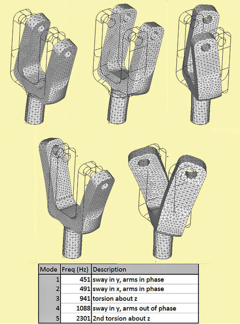 Fig. 2: Mode shapes, with description table.
The highest frequency may not be the dominating factor, so we also need to consider the loading. A sad case is a sharp shock input and a calculation time step that is bigger than the duration of the loading event. The FE analysis starts at the first calculation time step, and sadly it is all over before it has begun. This is a common beginner’s error. I have done it many times and wondered why no response occurs even though the FEA model and spatial loading are correct. (I reran our model with time step value for ms, not seconds, and so missed the loading.)
In general we must be careful to make sure that we capture the fidelity of the loading input. The peaky nature of a triangular or square input actually implies very high-frequency content. Remember the Fourier Series? It takes lots of sine terms to match these shapes. The load smearing effect described implies that using just a few points to follow the triangle will transform its shape and amplitude. It is better to be conservative with the time step in this case, using 50 or so time steps for the duration of the shock. Check the response at the input point to make sure the fidelity is preserved. Similarly, if the loading point is being driven at 1,000Hz, we need at least 0.1 ms time step size.
 Fig. 3: Modal Effective Mass table (translational).
If inputting a sine or cosine time-based loading form, look for a direct analytical definition in the solver, rather than a data table. The data table input relies on interpolation. Imagine five points used to describe a half-sine pulse. The FEA solver linearly interpolates between each point, so we get a poor definition of the input signal. An analytical input definition means that the interpolation is being done inside the solver to the accuracy of the time step.
The smaller the value of time step, the more accurate the numerical displacement differentiation will be, which may override the previous considerations. In a large model, decrease time step at a period of critical interest (say under impulsive loading) and increase it later. However, for linear transient analysis, changing time step can be CPU expensive. Normally it will take a few runs to tune the model overall, and the effectiveness of the solution technique can be investigated.
Number of Time Steps, Duration of Analysis
The number of time steps to be used in the analysis is important. Don’t guess on this or the time step size, as there is a logical approach. We want to capture enough of the response time history to make sure that any secondary swings after the initial response are captured. With complex mode shapes and phasing, it may be that the peak response occurs at some point in the history. Our aim is for the response to be clearly decaying at the analysis cutoff point, with no surprises later. Typically three or four free cycles of the lowest frequency content should be allowed to occur. The lowest frequency in the model and its time period should be straightforward to assess. From this, and the loading duration, the total duration of the analysis can be calculated. Knowing the time step size, we can calculate the number of time steps. In our case the lowest frequency is 451Hz , so each cycle is 2.22 ms; we need four cycles, so the free response should take 8.88 ms; the loading was on for 1.0 ms, so the total duration is 9.88ms. With an analysis time step of 0.0435 ms, this gives 227 steps. We can round this to 0.04 ms and 250 steps.
Data Output
The modern FEA trend is toward very large numbers of DOF. A transient analysis may have thousands of time steps. The potential to output Big Data is considerable. A useful approach is to consider two streams of output. One stream is for the big picture, an animation of the full response. Only a relatively few number of plot states are required to visualize this. If we have four cycles of a dominating low frequency response, with five plot states per cycle, then we can get down to a reasonable 20 complete sets of data. We probably need displacements at all nodes, but only need stresses on the surfaces of critical components. Careful consideration like this can make significant reductions in the amount of data stored and the time taken to transfer and display for post processing.
The second data stream is for detailed investigation by use of XY plots. There are key areas where we need a high fidelity to interrogate the frequency content and damping levels, frame these as if planning a physical test setup with data output channels. Requesting thousands of channels would be unpopular, so we settle for several hundred and probably focus on a few dozen. FEA is similar: Using engineering judgment and knowledge of the modal responses, we can predict the key points. Debugging a model using 20 output DOF, with 1,000 deflection and stress data points is extremely efficient. Investigate your post processing options carefully to see how you can set up these two data streams.
Response Investigation
The three key dynamic characteristics to investigate are listed below.
1. Check input loading.
Enforced motion analysis (applying displacement or acceleration directly) allows an exact comparison between input and response at the driven point. It is more difficult to check arbitrary external forces. We can, however, apply an equivalent static loading and check the level of displacement. This will give us a correlation to the dynamic response shape and dynamic magnification factor. At the very least, we can check the order of magnitude and duration of applied loading. In our model, the static deflection is 0.0465 in. laterally. The peak dynamic amplitude is 0.065 in. when loading ends at 1.0 ms. The dynamic magnification factor is 1.4, which is reasonable for a short pulse with a time duration less than the dominant frequency time period. The response is shown in Fig. 4.
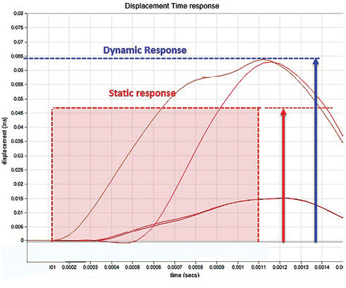 Fig. 4: Dynamic and Static response at loaded point.
2. Check frequency content.
We want to make sure that the model exhibits the correct modal characteristics under the loading actions. Many certification authorities demand this kind of evidence. Use key points in convenient directional responses to measure the dominant frequencies from the time history plot. This is done by picking off peak-to-peak time periods. One major advantage of using the modal method is that we can directly filter the modal content in the analysis to understand which modes are contributing. Fig. 5 shows the response of our structure with Mode 1 dominating and being tracked accurately.
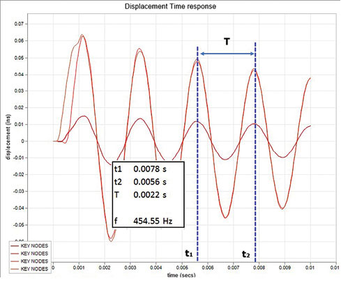 Fig. 5: Checking the dominant natural frequency.
3. Check damping levels.
We must confirm that the levels of damping defined in a model have been properly calculated during the analysis. There are several forms of damping simulation. Some of these can be problematic or error prone; Rayleigh damping depends on two coefficients in a quadratic equation, errors easily occur. Structural dumping relies on correct dominant mode identification because errors can badly affect damping levels.
We aim to find clean dominant modes showing decay after the loading is complete, under free motion. The log decrement method uses successive peaks to estimate the damping. The calculation for our structure is shown in Fig. 6, and the damping agrees with the input 2% critical value.
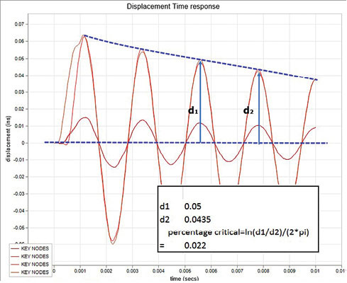 Fig. 6: Checking the damping level.
A Dynamic Story
The input parameters required for transient dynamic analysis can seem somewhat arbitrary, but there is a logical approach to estimating the time step size and the number of time steps.
There is a tendency to output an enormous amount of data in dynamic analysis, but with some planning you can keep the data down to a level required to do the job effectively.
Checking the dynamic response of the structure is vital. By using the key data point approach, we can investigate more deeply the structural response to loading input. Ultimately, we want to be able to “tell the story” of the structural dynamics.
More Info
Subscribe to our FREE magazine, FREE email newsletters or both!
Latest News
About the Author
Tony Abbey is a consultant analyst with his own company, FETraining. He also works as training manager for NAFEMS, responsible for developing and implementing training classes, including e-learning classes. Send e-mail about this article to [email protected].
Follow DE

