Figure 1: Yoke model; modes 1 to 4 and base driver in y direction.


Latest News
June 1, 2015
Editor’s Note: Tony Abbey teaches live NAFEMS FEA classes in the U.S., Europe and Asia. He also teaches NAFEMS e-learning classes globally. Contact [email protected] for details.
In last month’s issue of Desktop Engineering, we covered the basics of transient, or time-based analysis. This month’s article focuses on the alternative of frequency response analysis.
Frequency-based Response is not as intuitive as Time-based Response. We have to picture a virtual test setup with a shaker table that can be slowly driven through a frequency range. The table is infinitely stiff and our structure is rigidly connected to it at the constrained Degrees of Freedom (DOF).
We crank up the table and monitor as the oscillations are set at around 5Hz. In a non-simulation we have to wait until the response settles down to a steady state. In FEA (finite element analysis), we calculate the steady state directly and throw away the transitory response. At 5Hz we would plot a “frozen” response deformation shape that consists of all the peak amplitudes. We can also plot the peak accelerations, forces, stresses, etc. Having captured all of the results at 5Hz, we move on to 10Hz, capture all these peak responses, then move on to 15Hz and so on. We would go all the way up to the maximum frequency of interest, plus the safety margin we talked about last month.
Our virtual test results are a series of frozen displaced shape plots and all the corresponding peak response data at each frequency step. In a post-processor we can show each frozen plot shape and contour it with accelerations, stresses and more. More useful even, we can plot the peak responses at any DOF as a graph of response against frequency.
We are exploring an envelope of frequency input and plotting it as an envelope of frequency output. In other words, we are looking for trends across a range of excitation frequencies. A typical application would be a structure connected to a bulkhead or similar base structure, which is being shaken harmonically across a frequency range. This does not represent one physical event, but represents an exploration of the steady-state structural responses across a range of possible harmonic input loading that could occur during normal operation.
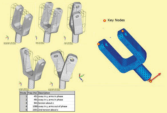
So far we have talked about shaking through the base of the structure—called “harmonic base motion” and there are many examples including Seismic excitation, a satellite attached to a launcher vehicle, or a car going over rough ground (although that has four independent “bases”). I am going to use the yoke model from last month and drive it laterally through its base, using Fig. 1 to remind us of the mode shapes and frequencies.
 Figure 1: Yoke model; modes 1 to 4 and base driver in y direction.
Alternatively, we can imagine a real test with point load introduced to the tip of a beam via a “stinger.” The stinger oscillates at a set frequency, and when the system settles to steady state, we measure the peak beam response. We change the frequency and repeat the process. This is called harmonic external excitation and we again can do this virtually in FEA.
The required input motion or loading amplitude versus frequency envelope can be a result of known loading characteristics (like the Seismic input or the satellite input). It can also be a constant amplitude sweep (often called a sine sweep), which explores the response of a structure under a ‘neutral’ input so as to understand the response characteristics. This latter effectively produces Transfer Functions that can be used in many applications.
This method has been used on the yoke. A unit 1g (386.4 in/s2^2) lateral acceleration is applied as a sine sweep to the base as shown in Fig. 1. The lateral (y) direction acceleration response graphs at the three key nodes are shown in Fig. 2.
 Figure 2: Frequency response plots of key nodes (acceleration).
Mode 6 response has been included for interest, even though it is outside our 2000Hz limit. Mode 1 and mode 6 were predicted to be the dominant players from the Modal Effective Mass (MEM) plot shown last month and repeated as an inset in Fig. 2. The MEM scale values should match exactly in base-driven Frequency Response analysis and are an important check.
Magnitude and Phase
One major complication in Frequency Response analysis is that in addition to the magnitude of the peak responses at each frequency calculation point, we also have a phase change. To give an idea of phase change, a single spring mass system has a single resonant or natural frequency. A driving harmonic oscillator is used as an input force. Below the resonant frequency the mass responds in phase with the oscillator. Above the resonant frequency the mass opposes the input force by being 180° out of phase. At the resonant point the phasing is 90°.
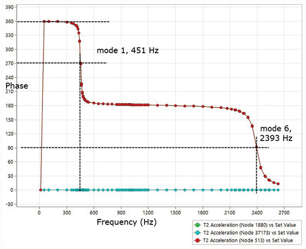 Figure 3: Phase response plot at key 3 nodes (acceleration).
All this means we have to input a forcing function in terms of magnitude and phase. Equally we have to plot a response in terms of both magnitude and phase. Fig. 2 shows the phase response plot for the yoke.
The two arms of the yoke start with an acceleration response phase of 360° (this is the same as 0°, i.e. in-phase with loading). As they pass through the first mode at 451Hz, they swing through 90° to 270°. Beyond the first mode, they settle at 180° out of phase. The next significant lateral y mode is mode 6 at 2393Hz. There is a further shift and a resultant in phase response beyond this mode.
The base-driven point as node 37173 stays fixed at the 0° phase, as expected.
If we try to plot the corresponding “frozen” response shapes, this can get very tricky. Almost all post processors will plot the response shape as a magnitude. We also need a phase interpretation to fully understand the implications.
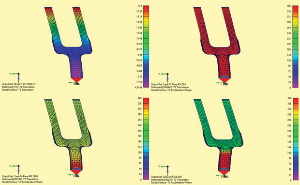 Figure 4: Phase change around mode 1 for acceleration response.
Fig. 4 shows four deformed shape plots. Fig. 4a is the first mode shape from the normal modes analysis. These should always be used to understand a response plot as they are a great guide.
Fig. 4b shows the phase as a contour at 424Hz – below the resonance. It is all red (360°). This ties up with our key point FR plot in Fig. 3.
Fig. 4c shows phase contour is changing at 451Hz (mode 1) and the arms turn cyan as they change phase to 270°. The base is still red at 360°.
Fig. 4d shows a swing to green (180°) at 500 Hz, beyond mode 1. Notice the response shape is changing and is drifting towards the next dominant y direction mode shape 6 at 2393Hz.
Now to really confuse you, mode 6 is plotted in Fig. 5a. What is going on?
The deformed shape plot can only work with magnitude, and remember this is only half the story. The phase is also plotted as a contour and shows the tips of the arms are blue at the 90° phase, as expected in Fig. 3 at mode 6 (2393Hz). The bottom half is cyan (270°) and there is a null or nodal line half way up at 180°. So, the tip and base of each arm rock about a mid-point, with a correct relative phase of 180°. I have “corrected” the plot in Fig. 5b.
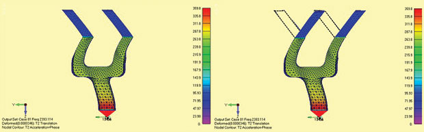 Figure 5: Mode 6 acceleration phase plots.
Frequency Response Calculation Points
Last month, I included a short sermon on the two approaches to any dynamic response analysis: direct and modal methods. To recap, a modal-based response analysis can get us answers cheaply, and help us understand the physics of the problem. It requires a normal modes analysis as the first step to generate the required mode shape vectors. The more expensive direct method can confirm the accuracy but strictly speaking doesn’t need any calculation of natural frequencies and mode shapes. However, we should do a normal modes (Eigenvalue) analysis anyway to get the natural frequencies and make sure we understand the physics.
We have another consideration in Frequency Response based analysis in that the accuracy of the solution is totally dependent on ensuring we do the response calculations at every natural or resonant frequency. The biggest responses are always at the resonant frequencies. Check mode 1 peak response in Fig. 2 and see how “spiky” it is. If we miss the natural frequency, we get the wrong non-conservative answer—simple as that.
There are various ways we can get the required natural frequency values in Hz into the FEA setup. Some solvers will automatically “slave” the Modal-based Frequency response calculation points using the values from the previous Normal Modes step automatically. Some require a Frequency input table that can be generated during a separate Normal Modes analysis. Another alternative is to use the pre-processor to capture results from a Normal Modes analysis and set up a table that can be included in the subsequent Frequency Response analysis. Getting accurate values into a Direct Frequency response solution can be a challenge.
Imagine the response in Fig. 2 as a pair of “hills” with “valleys” on either side. We have discussed hitting the peaks of these hills accurately. However we must also get a good spread of points around each peak to describe the hill accurately, and we must also add points to define the valleys adequately. There are standard schemes to do this. My favorite mix is 10 to 15 points spread +/- 10% around each peak and 10 points across each valley. The first—or left hand slope—is very important and I aim for around 15 there. The typical GUI (graphical user interface) controls are complicated, but I really recommend you master them as the accuracy is entirely dependent on this distribution of calculation points.
The hard way is to type the Frequency values into the input stream manually. This approach is both tedious and error prone, so you will need to find another way around. It may take some effort and guidance to figure out what steps are required for a particular FEA solver/pre-processor combo—but stick with it.
If we really overdo the points then we end up with a more expensive solution. However—it is far better than to have too few points or inaccurate points.
Response Investigation
I recommend two data recovery runs. One run to output a few full plot states to see the “frozen” shapes (maybe one of either side and at each resonance), and a second to output full data at the set of pre-ordained key points. As ever, this can save you a vast amount of data output.
The key dynamic characteristics to investigate are similar to the Transient Analysis.
1. Check input loading.
Enforced motion analysis allows an exact comparison between input and response at the driven point. Fig. 2 shows a constant base response of 1g (386.4 in/s^2) in y. It is easy to make mistakes in acceleration definition (for example 1 in/s^2 instead of 1g). I also failed to constrain my model correctly on the first run and had a gentle rotation towards infinity at low frequency that was spotted by checking the base motion.
2. Check frequency content.
Double check that the natural frequencies you predict at calculation points are still valid. Typical errors include pulling in the wrong set of Normal Mode tables, changing the model between the normal modes run and the Frequency Response run or using fixed instead of simply supported constraints.
Damping levels totally control the magnitude of the response. It is often good practice to run a Frequency Response analysis with two or three damping levels, then to show the sensitivity of the response to damping and ensure everyone is aware there is no “right” answer.
Meeting the Challenge
Frequency Response analysis requires a lot of digging in to fully understand what the analysis can reveal about the dynamic characteristics of your structures. To set the analysis up correctly takes some effort and is very error prone. Finally, the output interpretation can be challenging.
However, once you get the hang of it, it is a very important tool in dynamic analysis investigation. I recommend simple trial models of cantilever beams, two or three DOF spring mass systems and simple plates to get a feel for what is going on.
More Info
Subscribe to our FREE magazine, FREE email newsletters or both!
Latest News
About the Author
Tony Abbey is a consultant analyst with his own company, FETraining. He also works as training manager for NAFEMS, responsible for developing and implementing training classes, including e-learning classes. Send e-mail about this article to [email protected].
Follow DE

