

Latest News
May 9, 2018
Editor’s Note: Tony Abbey teaches both live and e-Learning classes for NAFEMS. He also provides FEA consulting and mentoring. Contact [email protected] for details.
This is the first in a new series of overviews that looks at finite element analysis (FEA) software products. Each overview will take the format of a walkthrough using a simple structural example. The full capabilities of each product can’t be covered in a few pages, but the intention is to give you a feel for the basic workflow required for each product.
Each overview represents my independent assessment. Please note that the companies developing the products do not sponsor the overviews. However, in many cases, I am indebted to the companies for supplying temporary licenses to allow the walkthroughs to be carried out.
FEMAP with NX NASTRAN Intro
The first overview in the series looks at the pairing of FEMAP and NX NASTRAN from Siemens PLM Software. The main emphasis will be on the FEMAP pre- and post-processing environment. The overview is in two parts. In this first part we will be covering the workflow up to meshing. In the subsequent part we will be completing the workflow through to post-processing.
You can view the complete model build in an online video.
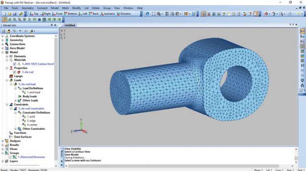
 Fig.1: The main FEMAP interface.
Fig. 1 shows the screen area, with a tie rod FEA model visible in the main graphics window. To the left of this is the Model Info pane. The “tree” view within this pane is currently showing the various FEA entities being built out that are ready for the analysis. At the top of the screenshot is a traditional drop-down menu that broadly follows the sequence of tasks in an analysis setup. You can either work exclusively from the drop-down menu, or use a hybrid approach with much of the functionality available in the more visual Model Info pane.
Below the main drop-down menu is the toolbar area with a variety of toolbars shown active. Again, you can work exclusively with the toolbars, or use a mix of these, the main menu and the Model Info pane in your workflow. A strong feature of FEMAP is the variety of approaches available. For an experienced user, this makes it a very rich environment. For the new user, it can be a bit bewildering; therefore, for the novices, the best advice may be to stay with the model info pane in the beginning.
However, even a new user will be tempted to set up tailor-made workflows very quickly, using a selection of the toolbars, or by beginning to create customized toolbars. The approach is similar to customizing toolbars in many Windows-based products.
The other default region in view is the Message pane below the graphics window. This provides continuous feedback for all actions you take, as well as various types of summary data.
There are a group of additional panes that can be opened to perform specialist tasks, such as meshing, post-processing and charting. We will be looking at some of these in the overview. The trend in FEMAP over the past few years has been to provide new or upgraded functionality via toolboxes located in these dedicated panes.
One thing to note in this overview is that I have changed many of the default entity and view colors to provide a clear set of images for the article.
Working with Geometry
Most users will be importing geometry into FEMAP. A wide range of formats is available, with advanced import settings for most of them. Fig. 2 shows the CAD model I have brought in, using the STEP file format. This CAD model is available for download in various formats.
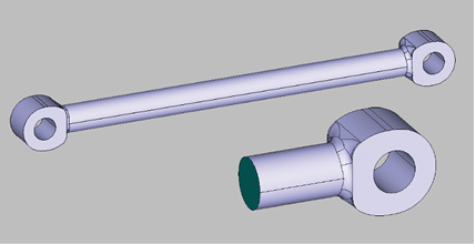 Fig. 2: Initial imported geometry and cut-out region.
Fig. 2 also shows the initial surgery applied to the CAD model. The component is symmetric, and the only area of interest from a structural analysis point of view is the fitting at the end. I have cropped the structure close to the end fitting. The stress state at the cut face is predictable, so this is a convenient approach to take. It avoids wasting resources on meshing and analyzing a large unwanted region of the component.
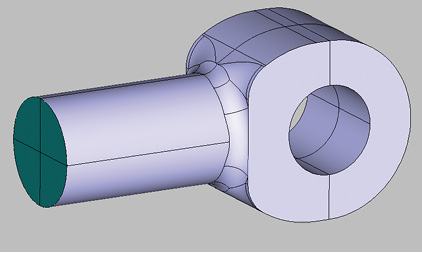 Fig. 3: Further manipulation of the geometry.
Fig. 3 shows the geometry after I carried out further manipulation. This provides surfaces on which to apply a bearing load. I also sliced the model vertically and imprinted a horizontal line on the cut face. The motivation was to provide better mesh control and allow clean edges for post-processing and a center point for one of the constraints.
The geometry manipulation took two forms: creating curves and projecting them onto surfaces, and then slicing the original body in two along a vertical plane.
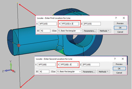 Fig. 4: Sequence of dialogue boxes to create a curve.
Creating curves and projecting onto surfaces to imprint is quite straightforward. However, there are several actions that are key to doing this efficiently. The first is a global control on what type of entities are picked using the cursor. The default is a screen pick, but right mouse-clicking on the graphics window allows this to be changed to select nodes (FEA entities), points (geometric entities) and other features. Setting the cursor pick to select points allows parametric manipulation within dialog boxes. For example, in Fig. 4 a vertical curve is created.
Point 108 is shown highlighted and is used as the reference point. The first end of the curve uses the XYZ coordinates of this point, but the Y coordinate is modified by +0.5. The second end of the curve uses the same point’s XYZ coordinates, but this time the Y coordinate is modified by -0.5.
Within any of the dialog boxes is a Methods option. This can change the way in which the dialog box operates. This provides a large variety of available techniques. In Fig. 4, the dialog boxes are asking for a location of each of the endpoints. For many dialog boxes, requesting a location will be the default Method. However, the Methods option can be changed to selecting the midpoint of the line, the center of an arc and many other shortcuts.
If another dialog box is used, such as deleting mesh, then the Methods options change and adapt to the task. In this case, useful Methods options include elements on specific surfaces, elements with a specific property ID and so on. This provides a workflow that is unique to FEMAP. Again, a newcomer to FEMAP will want to start exploring these options. Developing a personal set of tools from within this extensive toolbox is the goal.
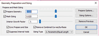 Fig. 6: Geometry preparation controls.
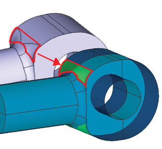 Fig. 5: Geometry preparation, combining surfaces.
At this stage, I carried out several trial meshes on the modified geometry. The transition region between the shaft and the end of the tie rod was very difficult geometry to work with. FEMAP has a powerful Geometry Preparation tool to address issues like this. This is essentially an automated geometry healing tool. Results of using the default settings are shown in Fig. 5.
The green colored surfaces, which I’ve highlighted, show a single surface created from the original surfaces. The thin slivers in the original surfaces were making them virtually impossible to mesh. The range of controls is shown in Fig. 6. Drop-down menus from this dialog box allow further advanced options.
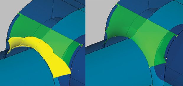 Fig. 7: Interactive cleanup of geometry.
FEMAP also has a dedicated Meshing toolbox that bundles together all the meshing controls and geometry manipulation controls found throughout the FEMAP menus. It also adds new functionality and provides an interactive view of geometry and mesh changes. It is evident from the functionality that the focus on geometry manipulation is to produce an improved mesh. An example of Meshing toolbox usage is seen in Fig. 7.
The left-hand side of the figure shows surfaces I’ve picked on the fly to combine together. I’ve also chosen the option to merge with existing surfaces. The right-hand side of the figure shows the result, with the surfaces now joined to the previous blended surfaces. Meshing is now much more controllable. FEMAP has a large buffer of undo levels, which can be increased if required. This means that exploring geometry changes and mesh changes gets easier. Users can undo mistakes.
Setting up Material and Physical Properties
Setting up material and physical properties to be used in the analysis is straightforward. Bear in mind that the traditional FEA data structure always links the material property to a physical property and the physical property is linked to each element. In the case of the beam or a shell element, this is intuitive. The physical property of a beam includes its cross-section and moments of inertia. The physical property of a shell will include its thickness.
The question becomes: What is the physical property of the solid element? Strictly speaking, it doesn’t have one in the same sense as the beam or the shell. However, the same linking data structure is used. In fact, the physical property of the solid element can be used to describe integration level and material coordinate system. In FEMAP it can also be used to allocate a color to the element. The latter has no meaning when translated into an input analysis file (traditionally known as the input deck), but can be used in various ways to reference the element within FEMAP.
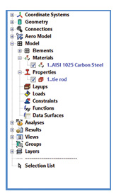 Fig. 8: Model Info tree view, showing Materials and Properties expanded.
Fig. 8 shows how I have used the Model Info tree view to define the material and physical properties. The tree can be expanded and contracted easily using the plus/minus symbols. Right mouse-clicking on an entity type, such as materials, allows new material to be created, and an existing material to be edited, deleted and more.
For models with many materials, physical properties and other entities, it is a useful way to be able to quickly survey what is present in the FEMAP database.
FEMAP provides a set of default material libraries, and the user can select from metric or US options. One word of warning: FEMAP, like many traditional FEA tools, assumes that the user will define consistent units—there is no global units setting. It is straightforward to build your own user library from within FEMAP. Each instance of the material in a FEMAP database is copied from the library. The material library exists as a text file and can be positioned in any convenient folder on your computer. The directory path to that folder can be modified within the FEMAP preferences. Material libraries can be shared between users on the same network.
Setting up Constraints
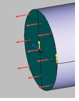 Fig. 9: The constraint system used in the tie rod model.
Fig. 9 shows the constraint system that is used in the tie rod model. The shaft at the cut surface shown here is restrained axially, but should be free to contract under the Poisson’s ratio effect. I have augmented the FEMAP screenshot with colored arrows to help identify the directionality of the constraints.
The constraint directions are color-coded with red as axial, yellow as vertical and blue as lateral. Three constraint sets exist: the first applies axial constraints to the four green surfaces, the second applies a single axial vertical and lateral constraint on the center point and a third applies a single vertical constraint on an edge point.
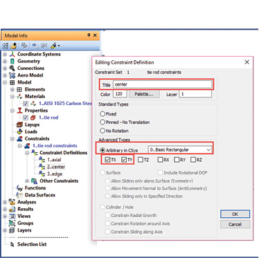 Fig. 10: The constraint sets and a typical dialog box.
The three constraint sets are shown in Fig. 10. They actually exist as subsets within an overall constraint set. This hierarchy helps with advanced analysis setup. The dialog box shows the result of right mouse-clicking on the center constraint definition and then electing to edit the form of the constraint. Alternatively, I could have chosen to edit the location of the constraints. The dialog box shows X and Y directions constrained in the basic coordinate system. If I had needed a local coordinate system, that could have been set up and chosen at this stage.
The constraints are applied to geometric entities. That is the preferred way of working within FEMAP because it allows independence from any subsequent meshing. However, FEMAP does permit direct allocation of constraints to nodal entities as an alternative. This can be useful in complex situations, but it does mean that a subsequent remeshing will destroy those constraints.
This parallel approach is common throughout FEMAP workflows. For example, it is possible to create a mesh without using any geometry at all. In difficult models it is sometimes convenient to develop a hybrid approach. A typical scenario would involve 95% of elements being meshed on geometry, and a really stubborn 5% being directly meshed.
This approach will be unfamiliar to those accustomed to a CAD-embedded FEA environment, but it reveals the legacy of tools such as FEMAP that existed before viable geometry was available.
Setting up Loading
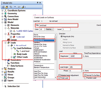 Fig. 11: The model Info tree view and the loading dialog box.
Loading is straightforward for the tie rod. There is just one axial bearing load applied at the connection end. The geometry was prepared for this, as described previously. The loading is created by right mouse-clicking on the tree view and creating an overall load set. From within this a subset is created. Fig. 11 shows the subset being created.
The option to use a bearing force has been selected, along with the magnitude of the loading and the angle over which the loading is going to be spread. In addition, it is confirmed that this load is a total value, rather than per surface. Load is defined as being normal to the surface. In addition to this dialog box, there is a further dialog box used to define the center point loading and the direction of the loading.
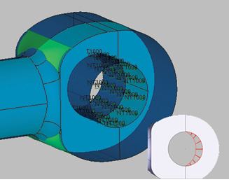 Fig. 12: Loading distribution created with inset schematic.
Fig. 12 shows the leading distribution applied over the selected surfaces. I have emphasized the cosine distribution in the inset schematic.
Coming up Next
In the next article, we will complete the analysis by meshing the geometry, running, and post-processing the results.
For More Info
Subscribe to our FREE magazine, FREE email newsletters or both!
Latest News
About the Author
DE’s editors contribute news and new product announcements to Digital Engineering.
Press releases may be sent to them via [email protected].


