
Fig. 1: Initial configuration and stress state.


Latest News
September 1, 2017
Editor’s Note: Tony Abbey teaches live NAFEMS FEA classes in the United States, Europe and Asia. He also teaches NAFEMS e-learning classes globally. Contact him at [email protected] for details.
In the previous article in this series (DE, June 2017), we looked at the SIMP (solid isotropic microstructure with penalization) method of topology optimization. In this article, we cover two other important techniques: evolutionary methods and level set methods. A wide variety of methodologies are used within topology optimization, as it is a rapidly developing discipline. Over the next few years there will many new developments with additional, or even combinations of, methods. It will be intriguing to watch the new products that this activity spawns.
Evolutionary Methods
The foundations of the evolutionary range of topology optimization methods begin with a fully stressed design approach as described in part 1. The concept is intuitive; any element with a stress level below a certain limit is eliminated from the model. The limit is expressed as a “Rejection Ratio.” The Rejection Ratio is the ratio of a threshold von Mises stress divided by a datum von Mises stress, typically yield stress. The threshold von Mises stress could begin at, say, 15% of yield and hence the initial Rejection Ratio of 0.15 is defined. If yield is 100,000 psi, then the first aim is to eliminate all elements with average von Mises stress less than 15,000 psi.
I have set up a demonstrator model using only linear static analysis. The model, loading boundary condition and initial stress state are shown in Fig. 1. The contour bands are set to highlight the threshold stress levels. The initial 15,000 psi level contour is marked on the image.
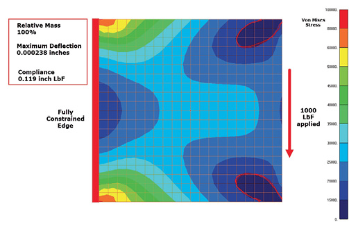 Fig. 1: Initial configuration and stress state.
Using a simple macro, the model is repeatedly updated by removing rejected elements until a configuration is reached, as shown in Fig. 2. At this stage, all remaining elements are above 15,000 psi von Mises stress. It took six analyses to converge to this state. The relative mass is now 86.5% and the compliance has increased from 0.119 to 0.132. In a simple case like this, the compliance can be estimated as:
(applied load) * (edge deflection) / 2
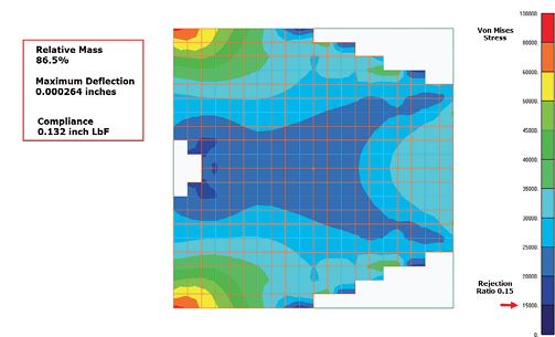 Fig. 2: Final configuration with initial Rejection Ratio of 0.15.
An important factor was that the region over which the load was being applied is shrinking. This is a common issue with topology optimizers; how should the load distribution be treated over a changing boundary? In this case, I manually updated the nodal load distribution to avoid eliminated nodes, being careful to apply equivalent kinematic loading.
I also found that eliminating elements completely gave bad convergence characteristics. So, I adopted the technique of reducing the stiffness of eliminated elements by a factor of 1E4, and retained them within the analysis. In commercial applications, other techniques are used to improve convergence. Indeed, one of the big advantages of the evolutionary methods is that elements can be fully eliminated. This means that as the volume of the material decreases, the number of degrees of freedom decreases and hence dramatic solution speedups can occur.
The Rejection Ratio is now increased, effectively increasing the target minimum stress throughout the model. The rate at which the Rejection Ratio is increased is called the Evolutionary Rate. I set the Evolutionary Rate to 0.05, so the next Rejection Ratio is 0.20. The target stress levels are therefore 20,000 psi, then 25,000 psi and so on. A further series of analysis is carried out, until convergence is achieved, with all elements above each new Rejection Ratio. It is clear from my simple experiments that a coarse Evolutionary Rate works well in the initial configurations, where there is plenty of material and relatively large stress variations. In the final configurations, there is little material, and stress variations are small. A much finer Evolutionary Rate is then appropriate so that the material is nibbled away more slowly.
Fig. 3 shows a montage of each of the converged configurations at Target Rejection ratios. It took 44 analyses to carry out the study. The trend is very logical and follows the classical benchmark problem. I have kept a constant maximum stress contour of 100,000 psi in the stress plots. It is evident that the component is becoming very overstressed at configuration 5. This occurs at a Rejection Ratio of 0.3; in other words no element has a stress below 30,000 psi. The volume is down to 43% of the initial configuration.
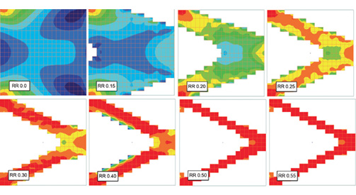 Fig. 3: Montage of configurations using the FSD (fully stressed design) approach.
The final configuration achieves 22.5% of initial volume and all stresses are above 55,000 psi. It is unlikely that this would represent a feasible practical solution, as the stresses are very high throughout the structure.
My topology optimization approach is very simplistic and not very representative of a commercial topology optimization strategy. However, it does show some of the representative features. Stress minimization is not a direct optimization strategy. The FEA model is an assembly of “LEGO brick” type elements, which do not attempt to model a continuous structural boundary. Mathematically, this approach is called the voxel method in 3D space. I used stress smoothing options to give a better sense of the stress flow. However, some of the configurations show the influence of the stress singularities that would be occurring in each of the internal corners. This can cause numerical problems in optimization methods. All topology optimizers will require a similar “one-eyed squint” at stress and material distributions to gain a sense of the configurations and their responses. In no sense are they representing a detailed stress assessment.
Fig. 4 shows the final configuration, with all material present, including the low modulus “chewing gum” type material. The full stress range is shown.
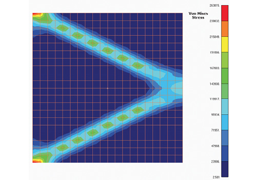 Fig. 4: Final configuration with all material shown.
The figure also shows another issue associated with topology optimization. The left-hand edge is fully built in. This over-constrains the model and will not permit Poisson’s ratio contraction to occur. It creates stress singularities at the top and bottom corners. This affects assessment of the structure, but could easily drive the strategy of a more sophisticated technology optimizer in the wrong direction. Yet the design intent of the configuration is clearly shown. That is really the objective of any topology optimization.
Commercial Evolutionary Implementation
Commercial topology optimizers do not use the fully stressed design approach directly. It is not applicable to more complex structures and requires development of ad hoc rules to keep it on track. Instead, it has been found that working with compliance gives more stable and manageable algorithms. Recall from my previous article that minimizing the compliance of a structure will maximize the stiffness. It is possible to derive the change in the compliance of the structure as a result of changing each element stiffness, for example, by dropping the stiffness from nominal material stiffness to zero, or to a very small value. This defines the compliance sensitivity of each element. Now, the evolutionary method can be modified to remove all compliance sensitivities below a certain level. The rejection ratio and evolutionary rate are defined as before, but now in terms of the compliance sensitivity. As we have seen with my simple model, slower evolutionary rates tend to give better convergence.
This approach is the essence of the evolutionary structural optimization (ESO) method. However, it is clear that this is a one-directional method. As in my simple example, there is no way of backtracking. As the configuration evolves, it may well be that deleted material should be replaced. If this is inhibited, then an optimum configuration cannot be found. In fact, unproductive dead-end configurations would be common.
The successor to the ESO method is the bidirectional evolutionary structural optimization (BESO) method. This uses various strategies to put back deleted elements as appropriate. The methods are similar to the smoothing and filtering techniques in the SIMP method that we reviewed in the previous article. The BESO methods focus on assessing the compliance sensitivities-per-element volume, similar to a strain energy density. The distribution of sensitivities densities can be smoothed and interpolated across voids created by deleted elements. If an interpolated sensitivity exceeds a threshold value, then the element is switched back on. The BESO method uses nodal sensitivities obtained by weighted average of the connected element sensitivities. This contrasts with the SIMP methods that use element sensitivities. The sensitivities are also smoothed across each successive pair of analysis to improve convergence.
The method can also introduce an element of “soft-kill,” in that elements are not fully deleted. This is done to avoid zero sensitivities associated with deleted elements. A small non-zero material stiffness is introduced instead and meaningful sensitivities can be calculated. A penalization method, similar to that of SIMP, drives material to the extreme conditions. However, the material distribution is still essentially binary, as opposed to continuously variable in SIMP.
The advantages of the BESO method include the fact that it is simple to understand as a heuristic process. It seems like a good idea to eliminate areas of low compliance, as this is understood to improve global stiffness. Because it is a hard-kill, or binary soft-kill, method, there is no gray area of intermediate densities. As long as the underlying voxel approximation to boundaries is appreciated, then interpretation of configurations is easier than the SIMP method. The computational speed-up, as elements and hence degrees of freedom are eliminated from the solution, can be very significant.
However, there are critics of the BESO method. Because it is a heuristic approach, it is difficult to identify any mathematical foundation and assess convergent qualities. Pathological test cases, where important load paths are deleted early on and never recovered, have been well publicized. However, the researchers in this field continue to develop strategies to overcome these issues, and it is currently a mainstream topology optimization technique.
The Level Set Method
There are several approaches to the level set method. The one described has evolved into commercial usage. A topological sensitivity parameter is established. This is a measure of the change in any structural response, based on the insertion of a small hole into the structure. The small hole modifies the topology. A high sensitivity means that any material removed, and hence the change in topology, will have a large effect on the response. On the other hand, low sensitivity means that there is little impact from the change in topology. If compliance is used as the structural response, then analytic definitions of the topology sensitivity can be established.
Directly removing elements that have a low sensitivity will result in the dispersion of deleted elements throughout the model, as we have seen in the SIMP and BESO methods. There is no inherent connectivity associated with the “holes” generated in the structure. The level set method takes a different approach and deals with that problem by mapping the overall distribution of sensitivity onto the mesh. Fig. 5 shows the concept behind the level set method.
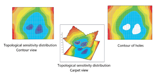 Fig. 5: The level set process.
Assume that the left-hand diagram represents an initial sensitivity distribution shown in a typical contour plot. The middle diagram shows how this can be viewed as a 3D carpet plot. The vertical axis represents the level of relative sensitivity. The 3D plot is clipped at a particular level of relative sensitivity. I have used the value of 0.3. The purple contour regions are below this threshold. The right-hand diagram shows these regions mapped onto the mesh and elements within this region are deleted in a contiguous manner. Essentially, interior boundaries are evolving. If the value of relative sensitivity is changed, then the clipping plane is changed, resulting in a different set of hole shapes.
The value of relative sensitivity is found by adjusting its value on the vertical axis, which changes the amount of material to be deleted. The aim is to match the current target volume fraction. Once the sensitivity level is found, the elements are deleted and the analysis is rerun. This results in a new distribution of sensitivity, and the fit is again made so that the topology matches the required volume fraction. After some iterations, the solution will converge to provide the relative sensitivity required to meet the target volume fraction. This interior boundary shape then represents the topology that provides the optimum compliance level at the target volume fraction. The method can also start from a configuration with inadequate material and grow material into the optimum topology.
Methods are used to evaluate elements where the boundary cuts through their volume. This is essentially a mass and stiffness smearing process. This is challenging in a 3D mesh and is the subject of continuing development.
Solutions to the Demonstrator Model
Fig. 6 shows the block used previously in my simple example, rerun in a level set method, with the same target 43% initial volume. The first run shown in Fig. 6(a) used a coarse mesh and the largest minimum feature size the optimizer would permit. A much more sophisticated result is produced! The configuration is 11% stiffer than my result. I reran with the finest mesh possible, with minimum feature size definition permitted. Fig. 6(b) shows that the result is even more sophisticated, with 14% increase in stiffness.
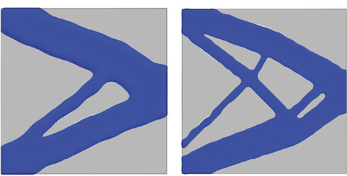 Fig. 6: (a) left, Level Set solution with small feature size. (b) right, even smaller feature size.
I also ran a SIMP-based solution, where I could force a “chunkier” minimum feature size, as shown in Fig. 7(a) and (b). The volume ratio was set at the same target 43%. Two variations on minimum feature size were used. The compliance was close to the Level Set method result in Fig. 6(a), in both cases.
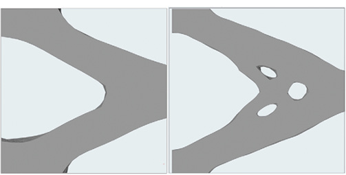 Fig. 7: (a) left, SIMP solution with large feature size. 7(b) right, medium feature size.
For a fair comparison in both cases, I also had to use the load footprint that developed in my crude FSD solution. The adapting load footprint is a tricky area, and I will talk more about that in part 3.
The Mathematics Behind the Scenes
The mathematics behind the topology optimization solutions can be very challenging. However, some understanding of the different processes available can give useful insight into how the methods are working behind the scenes. Perhaps the most important take-away from both articles in this series is that the configuration offered as an optimum solution is always an idea, rather than a fully defined structure. Often, the distinguishing features between topology optimizers are based on how this conceptual idea is carried forward into meaningful structure.
In the next article, I will look at more case studies using a variety of methods. This will include manufacturing constraints and development into final structural configuration.
Subscribe to our FREE magazine, FREE email newsletters or both!
Latest News
About the Author
Tony Abbey is a consultant analyst with his own company, FETraining. He also works as training manager for NAFEMS, responsible for developing and implementing training classes, including e-learning classes. Send e-mail about this article to [email protected].
Follow DE

