
Figure 5: Axial stress in conrod at 60° crank angle


March 1, 2017
How does load get into a component and how does it get out? Knowing the answer to these questions will help in setting up a good finite element analysis (FEA) simulation. Free body diagrams are one of the most useful tools in understanding load paths.
A free body diagram is a picture that shows all the external balancing loads acting on a component. It includes the set of applied forces and reaction forces and is used to check that all forces are in balance. For a 2D representation in an xy plane, there are three balancing equations developed:
1. Summation of forces in x (Fx);
2. summation of forces in y (Fy); and
3. balance of moment about z at some convenient point (Mz).
For a 3D representation in xyz space, there are six equations developed:
1. Summation of forces in x (Fx);
2. summation of forces in y (Fy);
3. summation of forces in z (Fz);
4. balance of moment about x at some convenient point (Mx);
5. balance of moment about y at some convenient point (My); and
6. balance of moment about z at some convenient point (Mz)
The general definition of what is a reaction force and what is an applied force is debatable. In an FEA model definition it is clearer, in a sense, as reactions are defined by constrained degrees of freedom and applied forces are defined through loading actions. So why the confusion? Well, the free body diagram is a more philosophical approach that tries to define the fundamental nature of the load path through the component. Figure 1 explains this idea.
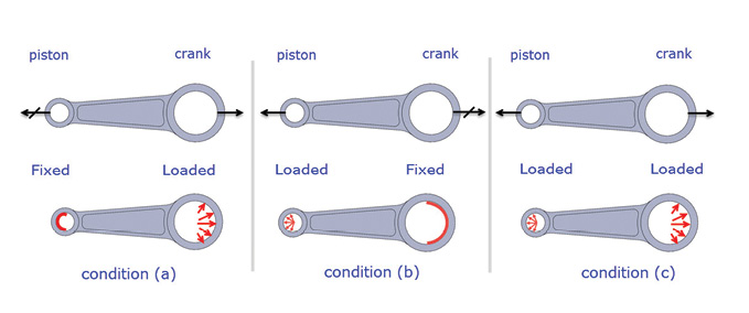 Figure 1: Alternative free body diagrams and FEA model sketches.
In Figure 1, condition (a), upper diagram, shows a conrod with an applied force at the right end (connected to the crank) and a reaction force at the left end (connected to the piston). The crank force is transmitted from the crank. The piston reaction is transmitted through the piston. The force and reaction vectors are drawn in a natural sense here, following their intuitive directions. Many industries also indicate a reaction by an oblique line through the arrow. The FEA model is shown in the lower diagram and uses the same boundary conditions.
Condition (b) shows a different interpretation of the same physical situation. The load is now applied at the left and reacted at the right. Both the free body diagram (upper) and the FEA load and boundary condition sketch (lower) shows this action. From a free body diagram point of view, it doesn’t matter which way we setup the action and reaction. However, from the point of view of a finite element analysis, it will make a big difference. Local stresses in the constrained regions for condition (a) or (b) will be very different and both will be inaccurate. A previous article, (“Free-Floating FEA Models,” February 2015) discussed the minimum constraint approach, and this is shown in condition (c). The FEA model sketch in Figure 1 clearly shows the load applied at both the right and left ends. The free body diagram shows the corresponding loads as actions, rather than reactions. In this case, the FEA model constraints are not shown. To stop rigid body motion, the minimum set of constraints (the ‘321’ set) must be applied.
All the free body diagrams shown in Figure 1 are correct: They show balance in the horizontal sense. Notice that a free body diagram does not include internal forces. We can look at internal forces separately, but the intention of the free body diagram is to show overall state of balance.
Conrod Basic 1D Equilibrium
So far, we have looked at the conrod component in a simplistic way. Loading is applied at one end and the opposite end is fixed, or we can use a minimum constraint approach. The first approach is used very commonly in basic FEA tutorials. A more realistic assessment looks at the overall physics of the piston and crank system and sets objectives for the analysis. The job of the conrod is clearly to transmit loading between the piston and the crank. There are two basic scenarios that occur. At the start of the power stroke, maximum gas pressure is exerted on the piston face. This is transmitted through the conrod and reacted at the crank. For now, we can assume the crank is locked against movement and hence will provide a complete reaction path to the piston force. This will be a compressive load path. On the return stroke, we can assume the gas pressure has dissipated and the piston is being accelerated with no resistance. Newton’s second law tells us that a force will be developed in the conrod as the crank resists this motion. This will be a tensile load path. Figure 2 shows these two scenarios.
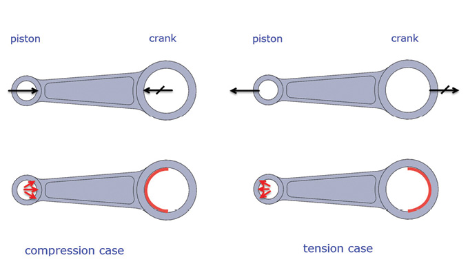 Figure 2: Compression and tension load cases in conrod.
A stiffness and strength assessment can be made based on these two loading scenarios. Fatigue analysis can also be carried out, assuming the stress range of each power cycle is defined by the compression and tension loadings. There are some more subtleties that could be applied, including inertia relief and friction effects. However, this is a common starting point.
Inertia Loading and 2D Equilibrium in the Conrod
There is, however, a big limitation in this method. We cannot get anything other than a one dimensional (1D) load balance from this system. The crank will rotate through 720° in a full power cycle, so it will spend most of its time in an off-axis configuration. We have only simulated top dead center and bottom dead center positions. How can we derive a free body diagram for an arbitrary crank angle?
The key here is to be able to define the inertia loading. That is quite tricky to achieve, and it is easiest to define both an acceleration diagram and a corresponding force balance diagram. Figure 3 shows the acceleration diagram of the conrod at some arbitrary crank angle. The accelerations are drawn relative to the conrod center of gravity (c.g.). The c.g. is at length r, along the conrod. The conrod sees an instantaneous rotational acceleration, alpha and longitudinal acceleration aA. There is also a centrifugal acceleration, r*w2, along the axis of the conrod which is due to the instantaneous angular rotation, w. Finally, there is a linear acceleration r*alpha. If the angular acceleration is ignored, then only the linear acceleration, aA, and the centrifugal acceleration, r*w2, exist.
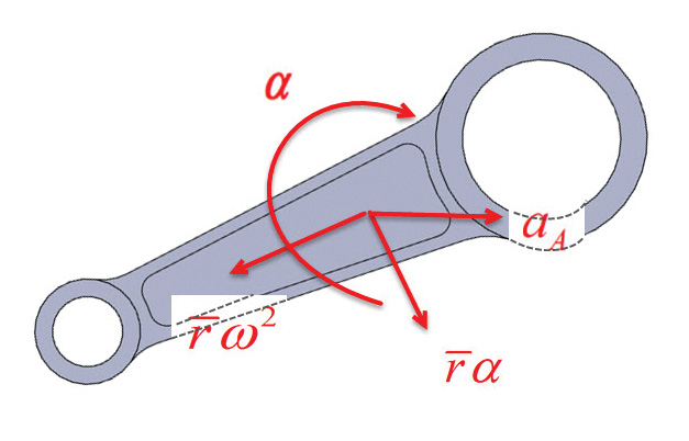 Figure 3: Conrod accelerations at arbitrary crank angle.
This example is well documented in reference 1 at the end of this article.
Having established the accelerations, the corresponding inertial forces can now be described. These are shown in Figure 4. The balancing forces at the piston and crank interfaces are also shown as forces F1 through F4. For convenience, the piston forces F1 and F2 are shown in the piston local axis system. The crank forces F3 and F4 are shown in the conrod local coordinate system. Any coordinate system can be used as long as balance is maintained in the free body diagram. The forces are balanced horizontally and vertically, and moments are taken about the piston end. All forces can now be calculated for this crank angle, given the gas pressure load, crank rotational speed and crank rotational acceleration.
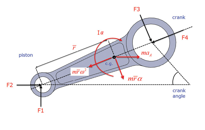 Figure 4: Conrod force balance at arbitrary crank angle.
What is interesting now is that we have reaction forces at right angles to the conrod axis—therefore bending loads can be sustained in this system of loading. The resultant bending stresses can be important in strength, stability and fatigue assessment. It is usual in this type of analysis to do a finite element analysis at positions all around the power stroke, spread throughout the 720° range to assess worst-case positions. It is also likely that a full kinematics analysis would be used with a multi-body dynamics simulation tool to provide the balancing forces, and accelerations for a given gas pressure history and crank RPM.
Figure 5 shows the axial stress distribution under the loading case shown. All loads have been applied as pressure distributions, or body inertia loads under translational and rotational accelerations corresponding to the acceleration diagram in Figure 3. The ‘321’ minimum constraint method has been used as described in the February 2015 “Free-Floating FEA Models” article. The crank angle is 60° from top dead center. There is significant bending overlaid on top of the compressive axial response. The use of a free body diagram allows the balancing forces and moments to be investigated and applied correctly. Without this, the conrod can only be analyzed with simple axial load cases.
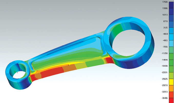 Figure 5: Axial stress in conrod at 60° crank angle
Sign Conventions
There are two main alternative conventions for loading on a free body diagram. Figure 4 used the natural orientations of the loads. This implies that we can predict the orientation and sense of the loading, and the sense of the vectors follows this. Consider the conrod under horizontal balance in Figure 6 (a). We can draw an applied load due to gas pressure coming into the small end and a force reacted at the crank through the big end. This puts the conrod into compression and we can write an equation where F1 equals F2.
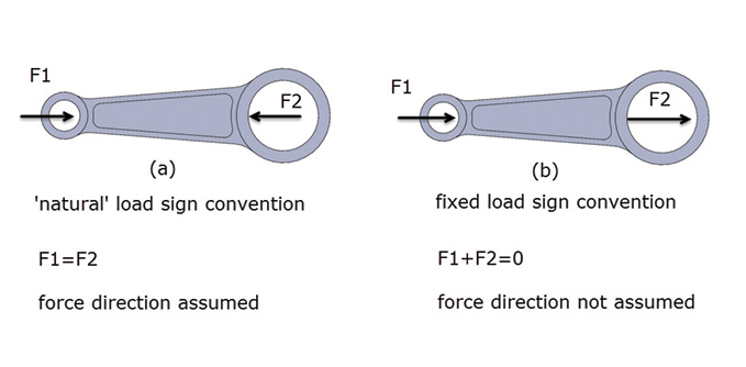 Figure 6: Load and force sign conventions.
Another approach is to take a fixed sign convention where we ignore any preconceived ideas about loading direction. This is useful when we are unsure of the loading or reaction sense. It avoids a situation where we’ve assumed a compressive reaction that turns out to be tensile load and we can end up with a double negative in the diagram! Figure 6 (b) shows F1 and F2 in a positive sense to the right. We then sum F1 plus F2 to zero: balance in the horizontal direction. F1 will equal minus F2.
Checking Load Paths
Many engineers are familiar with free body diagrams from their college days. The task then was to carry out a hand calculation and evaluate all the forces in a structure. One of the reasons that we typically avoid doing this in practice is that most structures have redundant load paths (i.e. are statically indeterminate). The equilibrium equations: three in 2D problems six in 3D problems are not enough to solve the structures, so we use energy methods, such as FEA. Figure 7 (a) shows a cantilever beam, which is determinate and can be solved by hand. However, if we introduce one redundancy as shown in Figure 7 (b), then we must use energy methods to solve. Adding a moment restraint in Figure 7 (c) means there are two redundancies—and more tedious work to do.
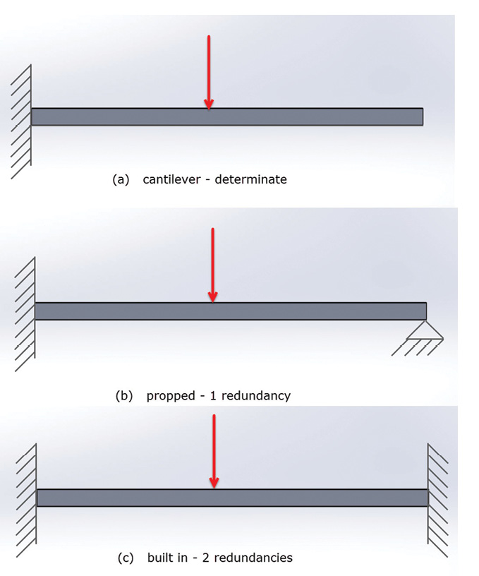 Figure 7: Beam free body diagrams.
For a typical component, we are not attempting to do the stressing by hand—we use FEA. Now the free body diagram acts as a very useful tool to check the load balance. The actual distribution of loading will depend on the relative stiffness of the load paths. The bracket shown in Figure 8, is loaded with 1,378 lbf resultant vector acting in an off-axis direction. The load is reacted at three bolting positions. The assumption is that only translational forces are reacted. A free body diagram tool is used to post process the results and show the nature of the reaction forces.
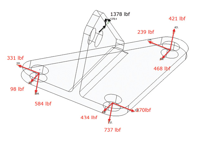 Figure 8: Free body diagram of reaction and applied forces in bracket.
One observation is that the two rear bolts act to resist the load in axial tension (584 lbf and 737 lbf), the front bolt resists with axial compression (-421 lbf). The model would be improved if an attempt was made to model the bracket bottom plate bearing footprint under the front bolt region. Bolt shear actions can also be checked and design decisions made. The free body tools can be complicated to set up in a post processor, but they are worth pursuing as they give definitive answers. The Von Mises stress distribution is also shown in Figure 9.
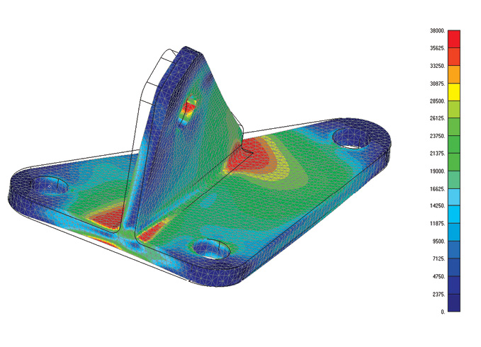 Figure 9: Von Mises stress distribution in bracket.
It is important to understand the nature of the loads that a structure carries. We can consider them either as applied loads or reaction forces. Drawing the diagram manually, or from FEA results, permits a clear picture of the load balance—both for checking and for design assessment.
In a future article, I will look at checking internal load balance, using typical FEA post processing tools.
Reference1. Mechanics Part II: Dynamics. J.L.Meriam 7th. Ed. Wiley 2012. ISBN-13: 978-0470614815
Subscribe to our FREE magazine, FREE email newsletters or both!
About the Author
Tony Abbey is a consultant analyst with his own company, FETraining. He also works as training manager for NAFEMS, responsible for developing and implementing training classes, including e-learning classes. Send e-mail about this article to [email protected].
Follow DE

