
Fig. 5: A nonlinear structural analysis with direct thermal loading.


Latest News
June 1, 2014
Editor’s Note: Tony Abbey teaches live NAFEMS FEA classes in the US, Europe and Asia. He also teaches NAFEMS e-learning classes globally. Contact [email protected] for details.
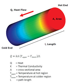 Fig. 1: Conduction along a rod.
When figuring out thermal problems, engineers can draw from a variety of solutions. These include finite element analysis (FEA), finite different approaches, 1D thermal networks and thermal analysis within computational fluid dynamics (CFD) solutions. This article concentrates on the FEA methods with an emphasis on thermal analysis used in support of, or in conjunction with a structural FEA analysis.
The extension from a structural FEA solution to a thermal FEA solution is quite straightforward as there are direct analogies between the variable we are solving for—displacements become temperatures, and the terms in the matrices we are building—stiffness becomes thermal conductivity, and the full analogy between structural and thermal modeling is shown in Table 1.
Table 1 also shows both US and SI systems of units. SI thermal units are straightforward, US thermal units can be confusing with “hard wired” time and distance terms. It is a good idea to check in a thermal textbook for simple examples of units and to practice and double check working with them.
Structural | SI | US | Thermal | SI | US |
Displacement | m | in | Temperature | K | F |
Stress | N/m^2 | Lbf/in^2 | Heat Flux | W/m^2 | Btu/hr.ft^2 |
Load | N | Lbf | Heat | W | Btu/hr |
Stiffness | N/m | Lbf/in | Conductivity | W/m.K | Btu/hr.ft.F |
m | meter | K | Degrees Kelvin | W | Watts |
in | inch | F | Degrees Fahrenheit | Btu | British thermal unit |
N | Newton | Lbf | Pound Force | hr | Hour |
ft | foot | Table 1: Structural and thermal equivalents in US and SI systems. | |||
Going back to basics, we are considering three types of heat transfer: conduction, convection and radiation. The physics of each of these and implications for the FEA solution are discussed in turn. The heat transfer equations for each are shown in Figures 1, 2 and 3.
Conduction Considerations
Conduction occurs when there is a temperature differential across a component. The heat energy will flow from the hotter region to the cooler region. The heat energy depends on the temperature differential, the cross sectional area of the material in the component and the thermal conductivity of the component material—all in a direction normal to the energy path. It is inversely proportional to the path length.
Material US Units | (Btu/hr.ft.F) | SI Units (W/m.K) |
Air | 0.0153 | 0.026 |
Glass | 0.50 | 0.865 |
Nylon | 0.14 | 0.242 |
Styrofoam | 0.02 | 0.035 |
Al 2024 T4 | 70 | 121.1 |
Titanium | 9 | 15.6 |
Pure Copper | 230 | 398.0 |
Steel SAE 1010 | 34 | 58.8 |
Table 2: Conduction coefficient for various materials (US and SI units). Do not use as definitive – check sources. | ||
If we think of a round bar, say 1 m in length, it is intuitive that we will be transferring more energy if the temperature differential is 200°C rather than 100°C. Similarly if the bar is of radius .025 it will transform less energy than a bar of radius .05 m. Thermal conductivity is a material property. Highly conductive materials include copper, while low conductivity materials include ceramics. The bar in our example if made of copper, will transmit much more thermal energy than a ceramic bar. Table 2 shows typical values of thermal conductivity. Finally, consider the bar shortened to 0.5 m. With the same temperature differential the heat flow will be doubled.
Forms of Convection
Convective heat transfer from a surface occurs by movement of the adjacent gas or fluid, such as air. Convection typically transports warmer fluid away from the surface and replaces it with cooler fluid. The actual mechanism of the fluid movement is quite complicated and involves a boundary layer at the surface that permits local thermal transfer by conduction. This thin layer then circulates away from the surface and is replaced by a fresh layer of cooler air. The micro level of transportation is simplified into an effective macro representation, which is assumed dependent on the temperature difference between the surface and the free fluid, the surface area and the convective heat transfer coefficient.
[gallery columns=“2” ids=”/article/wp-content/uploads/2014/06/Figure2_Natural_convec_opt.jpg|Fig. 2: Natural Convection from a surface.,/article/wp-content/uploads/2014/06/Figure3_Forced_convect_opt.jpg|Fig. 3: Forced convection from a plate surface.”]
Because convective heat transfer relies on fluid motion, there are two basic forms. The first is called free convection in which the fluid is initially stationary and then is assumed to circulate because of the local heating. The orientation of the surface with respect to gravity is important here; if the surface is vertical then gravity is assisting in the motion of the fluid. If the surface is horizontal then gravity will not initially assist the circulation. Figure 2 shows a schematic.
There are many standard methods for estimating the free convection heat transfer coefficient.
An alternative form of convective heat transfer occurs when the fluid is being entrained to move by some external driving force. For example, a fan blowing across a surface as shown in Figure 3 will provide a more energetic medium for the fluid to move away from the heated surface. Calculating the actual heat transfer under forced conditions can be very complicated and for accurate solutions may require a coupled CFD analysis. There is some variability also as to where the surface temperature and the free strain temperature are measured. However, luckily for us for many empirical calculations are available to estimate the convective heat transfer.
Radiation Calculations
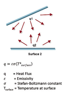 Fig. 4: Radiation between two surfaces.
Any surface which has a temperature above 0° Absolute is theoretically emitting heat energy by radiation. The transport mechanism in this case is by electromagnetic waves or photons emanating from the surface. This mechanism does not need a medium to pass through, so radiation can occur in a vacuum. As well as emitting radiation a typical surface will also be absorbing radiation from adjacent surfaces or sources. Emissivity and absorptivity are properties of the surface. The relative temperatures of each surface, absorptivity, emissivity and the angles at which the photons track between them will govern whether an individual surface is cooling or heating.
There are several difficulties associated with radiation calculations, the first is that the view that panel A has of panel B controls the tracks the photons can follow between the two panels. This parameter is called the view factor and can be very difficult to calculate for arbitrary surfaces, without some kind of ray tracing solution. Luckily for us, many common surface shapes and orientations have empirical solutions. A further very important aspect of radiation is that the heat transfer is dependent on a fourth order temperature term as seen in Figure 4. This means that any heat transfer analysis including radiation effects becomes a nonlinear solution.
Four Types of Analysis Solutions
- Linear solutions. In a linear solution the material thermal properties do not change with time or temperature and there is no radiation. It can be confusing in some solvers to define a linear solution, as the default solution strategy is nonlinear, and will only revert to a linear solution in the absence of radiation and other nonlinear effects.
- Nonlinear solutions. In a nonlinear solution the material thermal properties can vary with temperature. Thermal boundary conditions and loading can also vary with temperature. As mentioned, the presence of radiation will force a nonlinear solution. Examples of nonlinearity include thermal conductivity, convective heat transfer coefficient and applied heat flux from the source as a function of temperature. Nonlinear analysis requires a load incrementing strategy with the total thermal loading broken down into successive steps. This is exactly analogous to structural nonlinearity.
- Steady-state analysis. The steady-state in a thermal event occurs when the temperature distribution and all thermal flows stabilize and remain constant through time. The steady-state can be calculated directly by performing an energy balance assuming this stabilized condition. Steady-state conditions are often of interest to derive a temperature distribution over component, which is then used in a subsequent structural analysis.
- Transient analysis. In this type of analysis the initial conditions are defined and then time stepping solutions carried out in response to the thermal loading and boundary conditions. The calculation can be carried out through to a steady-state condition, or to evaluate initial thermal shock loadings, for example where the steady state condition is not important. One of the considerations in the transient thermal analysis, somewhat analogous to a transient dynamic analysis, is an accurate calculation of the time step required. In the thermal case there is a stability criteria that is often used to establish what this should be. It may be that the solver uses this time step automatically, or the user has control to set up one’s own time step. Time steps coarser than the stability limit are not advised. In some analyses the rate of change of thermal effects is dominant in the beginning of the analysis, so time steps here will be critical. In other analyses a nonlinear effect may occur well into the time history and require fine attend steps. Many solvers have adaptive time stepping that can, to some extent, deal with this variation in optimum time step.
Thermal Strain Loading in a Stress Analysis
As mentioned, in many cases, the thermal analysis objective is to provide the temperature distribution for subsequent stress analysis. In a typical uncoupled thermal and structural solution, a steady-state temperature distribution is mapped from the thermal model to the structural model. Mapping can be direct within the same physical mesh, or interpolated between dissimilar mesh models. Either approach will result in thermal strains throughout the structure. The thermal strain is proportional to the temperature change from initial conditions and the coefficient of thermal expansion. If a component such as a bar is allowed to freely expand under a uniform soak of temperature change then it will have a constant thermal strain throughout and there will be no stresses induced. However, if both ends of the bar are held, then the thermal strains are opposed by induced mechanical strains—the bar is not free to expand naturally. In practice components will have a more complex temperature distribution and distribution of thermal properties as well as mechanical boundary conditions and will develop thermal stresses throughout, even if nominally free to expand. A simple example of this is a bimetallic strip.
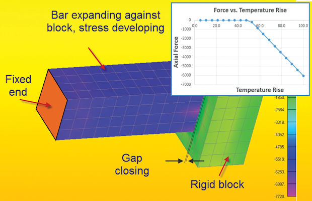 Fig. 5: A nonlinear structural analysis with direct thermal loading.
Figure 5 shows a bar that is free to expand in a stress free manner until a small gap is taken up with an adjacent block. At this point the stresses will increase from zero. An initial thermal analysis is not needed in this case as the temperature field is just a constant elevated temperature which is defined as a thermal loading in a structural sense directly into the stress analysis. However as the gap is closing a nonlinear static solution is required.
Material structural properties can be temperature dependent, but still allow a linear static solution and steady state. The temperature dependency is essentially a lookup table for each material structural property at a specific temperature. It does not matter if the actual temperature dependency is linear or nonlinear.
A nonlinear static solution may be required if the thermal loading means that linear structural responses are exceeded. This could include regions of plasticity or material nonlinearity, or geometric effects such as large displacement, buckling or contacts (as seen in Figure 5). A judgment is needed here to decide whether a fully coupled solution should be attempted—where both thermal nonlinearity and structural nonlinearity are updated throughout the analysis. A simple example would be opening or closing of contacts changing the thermal load distribution.
Solution Accuracy and Applicability
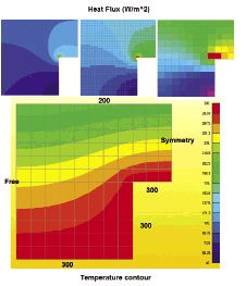 Fig. 6: Thermal singularity in sharp corner shown by Heat Flux contours.
Just as in structural analysis using the FEA method, thermal solutions can also suffer from various inaccuracies. The FEA solution is always a discretization of a continuous response. In structural analysis the response is the displacement field, and a thermal analysis it is the temperature field. We usually assess the accuracy of structural analysis by looking at stress jumps between adjacent elements and attempt to achieve a convergence. When considering thermal analysis, the temperature distribution is the most commonly presented form of thermal response, typically as a contour plot. However, to obtain a better feeling for how accurate the solution is, we should really be looking at the heat flux passing through each element—this is analogous to the stress in the structural solution and hence is a good indicator of convergence and accuracy. A classic example is the simple structure shown in Figure 6. The sharp corner is in fact a singularity both in the thermal and structural sense. This is not so obvious when looking at temperature distributions, but does become obvious when looking at heat flux distributions as shown in the top right inset. Heat flux distributions are not so intuitive as the stress distributions so they tend to be ignored other than at boundaries. The figure also shows a mesh refinement study—the singularity does not go away, but its effect is reduced, and the overall accuracy of the heat flux distribution, is vastly improved.
Comparison with structural analysis is useful when thinking about other sources of inaccuracy. We know that constraining the structure is a harsher boundary condition than applying an equivalent pressure loading when trying to simulate connection to an adjacent component. A judgment has to be made as to which method is more appropriate or whether we should be thinking about using boundary stiffnesses or contact surfaces. The same applies to a prescribed temperature on a boundary as opposed to a heat flux passing through boundary. They may both develop the same effective thermal loading but one will be harsher than the other.
If the objective of thermal analysis is to provide temperature distribution for subsequent structural analysis, then it is worthwhile to investigate the sensitivity of that structural analysis to errors in the thermal distribution. That is the ultimate measure of required accuracy.
Challenging Analysis
Thermal FEA solutions are relatively straightforward to set up, however obtaining the required accuracy, idealization methods and mesh discretization can be challenging. A smooth temperature contour plot is not a very good indicator; instead the heat flux convergence is a better guide and is analogous to the stress convergence in a structural solution. If the ultimate goal is a structural analysis with thermal strain loading then the accuracy and sensitivity of this analysis with respect to the thermal modeling is the criterion to judge the analysis by.
Subscribe to our FREE magazine, FREE email newsletters or both!
Latest News
About the Author
Tony Abbey is a consultant analyst with his own company, FETraining. He also works as training manager for NAFEMS, responsible for developing and implementing training classes, including e-learning classes. Send e-mail about this article to [email protected].
Follow DE

