

Latest News
November 1, 2016
I was teaching an “Introduction to Finite Element Analysis (FEA)” training course in the Netherlands recently. A design engineer taking the course came up with a good question relating to a graph I had just sketched up on the whiteboard. I was describing how a material would respond to the loading, in terms of its stress and strain, as shown in Fig.1.
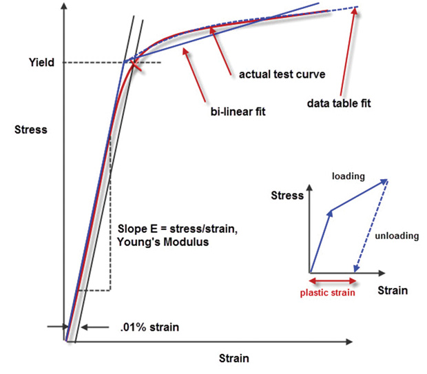 Fig. 1: Hooke's Law
I had described the linear part of the graph as representing Hooke’s Law, and then overlaid a triangle to show that the slope of the linear region of that curve is Young’s Modulus. My questioner wanted to know “Why not Young’s Law and Hooke’s Modulus?”—the two seemed interchangeable. Well, the question underlined how easy it is to get confused between the context of the two definitions. So let’s rewind, and think how I could’ve presented this in a better way.
Robert Hooke’s Watch Springs
Robert Hooke (1635-1703) was the first of the two English gentlemen whose names we are considering. His experiments looked at the relationship between an applied force and the subsequent extension, using structural components. These were mainly simple linear or rotational springs. He was able to show that the relationship between the force and the resultant extension was linear over a large operating range. In particular, he was interested in the application of this to the response of helical watch springs. In fact, his clock inventions formed the basis for a lot of his early wealth.
Hooke’s Law is therefore applied to structural components, from simple linear or rotational springs to much more complicated structures.
Application to Structures in FEA
For a rod under axial loading we can show quite easily the stiffness of the component rod is AE/L, where A is the cross-sectional area, E is Young’s modulus and L is the length. So we can use Hooke’s Law to derive F=k*d, or F=(AE/L)*d, where k is the rod axial stiffness, F is the applied force, and d is the deflection we solve for. The graph is shown in Fig. 2. This is a single degree of freedom (SDOF) solution.
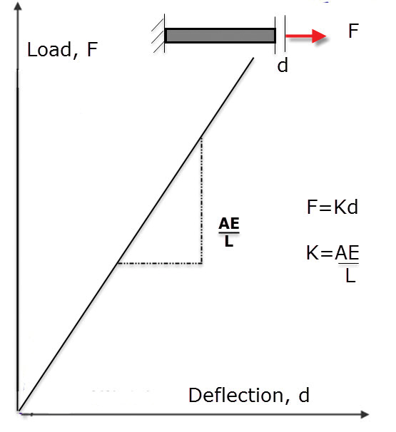 Fig. 2: Hooke’s Law: Load vs. deflection for rod.
In an FEA simulation more complex structures, with many DOF, are loaded. The complete load vs. deflection relationship is defined by the system stiffness matrix. The system stiffness matrix is derived by assembling the stiffness matrix of all the elements. So now {F}= [K]*{d}, where {F} is the applied load vector, [K] is the system stiffness matrix and {d} is the vector of deflections we solve for. The complete structure follows Hooke’s Law. We can in fact break out a single degree of freedom (SDOF), for example at a key deflection. If we plot the total load vs. deflection at this point, we can see Hooke’s Law in action, as shown in Fig. 3.
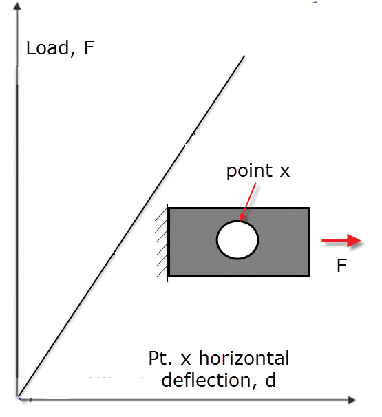 Fig. 3: Hooke’s Law: Structural stiffness of component.
We can even evaluate the equivalent SDOF stiffness of a structure by loading that point and measuring the deflection, as shown in Fig. 4. This will now be analogous to the response of an equivalent spring stiffness. This is a useful method of assessing structural component stiffness in design. This technique allows us to compare load paths within a structure, create boundary conditions, estimate modal stiffness and has other applications.
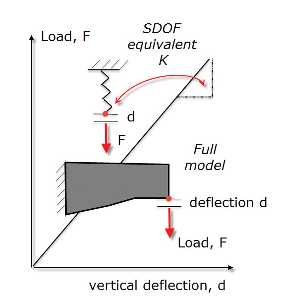 Fig. 4: Equivalent SDOF stiffness of structure.
Thomas Young and Elasticity
So how did Thomas Young (1773-1829) get involved? He was concerned with the elasticity of the material itself. So this is much more specific than the general Hooke’s law (which still applies). The linear relationship of the material is what we call Young’s Modulus. He was one of the first researchers to realize that each type of material has its own inherent stiffness, and the relationship is named in honor of him.
The graph in Fig. 1 shows a typical uniaxial (1D) test result to evaluate Young’s Modulus. A more general 3D stress strain relationship can be derived for Isotropic materials by using Poisson’s ratio. This relates the axial strain to the transverse strain.
Hooke’s Law is an overall structural stiffness term, dependent on the configuration, as well as the inherent material stiffness properties; whereas Young’s Modulus is specifically the stiffness of the material itself.
So, to use the phrase from the old Abbott and Costello sketch—in our team, Hooke’s on First!
Subscribe to our FREE magazine, FREE email newsletters or both!
Latest News
About the Author
Tony Abbey is a consultant analyst with his own company, FETraining. He also works as training manager for NAFEMS, responsible for developing and implementing training classes, including e-learning classes. Send e-mail about this article to [email protected].
Follow DE

